50.6k
50.6k
Another month goes by, which means it’s time for another release!
The ClickHouse 26.7 release contains 61 new features 🌻 112 performance optimizations ⛱️ 329 bug fixes 🍉
This release brings speedups for GROUP BY ... ORDER BY ... LIMIT, three JOIN improvements, faster vector search with QBit, position-aware phrase search, EXPLAIN ANALYZE, unified URL access, and more!
New contributors
A special welcome to all the new contributors in 26.7! The growth of ClickHouse's community is humbling, and we are always grateful for the contributions that have made ClickHouse so popular.
Below are the names of the new contributors:
Aditya Kumar, Ali Ayman, Andre Murbach Maidl, Antonio Álvarez Caballero, Arbin, Arup Chauhan, Bala Vignesh S, Blackmorse, ClickGap Bot, David Meng, Din, Eduardo Gomez Saldias, GalBenMoshe, Gaurav Dubey, Goutam Adwant, Jitendra, Keguang Xu, Kermit, Lalit Yadav, Manuel Cadarso, Maoyao233, Matheus Agio Nerone, Mihir G, Murphy, NIKTONIKTO717, Oranje AI, S Bala Vignesh, SBALAVIGNESH123, Samuel Krempaský, Sayantanu Dey, Stack Slayer AI, Tamish Mhatre, Umang Agrawal, Vismay, Yang Hu, Yanjun Qiu, adityaksolves, ashishch432, cadarso77, clickhouse-docs-bot, clickhouse-robot-gh, coderashed, fidelaggio, gaurav0107, jaehanbyun, jitendra, jordiori, kgeg401, lefteris gilmaz, linhaojie, lzp, malgamves, mintlify[bot], motsc, slach, unintended, vismaytiwari, wandersofb, ymy
Hint: if you’re curious how we generate this list… here.
You can also view the slides from the presentation.
Faster GROUP BY ... ORDER BY ... LIMIT
Contributed by Konstantin Bogdanov and Nihal Z. Miaji
Top-N queries are everywhere in analytics:
“Show me the latest events.”
“What are the most expensive orders today?”
“Return the first 10 results in key order.”
They all share a familiar SQL pattern:
... ORDER BY ... LIMIT NClickHouse treats Top-N as a first-class query pattern. Over time, the engine has accumulated several complementary optimizations, including streaming execution, read-in-order, lazy reading, and granule-level data skipping.
Why GROUP BY normally reads everything
But what happens when ClickHouse must aggregate the rows first?
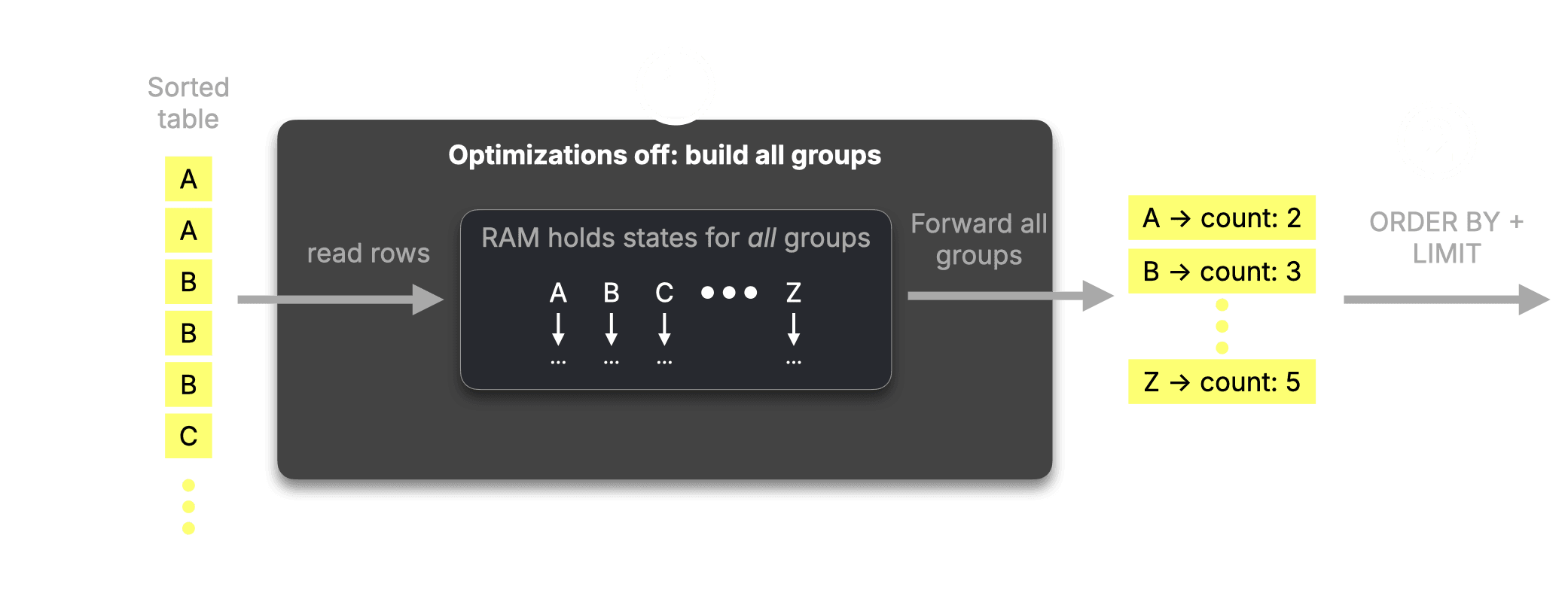
Without exploiting the table’s order, a conventional GROUP BY must ① keep every group in memory until all rows have been read. For example, with count(), ClickHouse keeps every key and increments its count whenever another row with the same key appears. Only then ② can ORDER BY ... LIMIT discard all but the first N groups:
The first step: GROUP BY ... LIMIT without ordering
In 26.5, we optimized one version of this pattern: GROUP BY ... LIMIT without an ORDER BY. ClickHouse still scans the input, but keeps only N arbitrary groups in memory.
Two optimizations in one fused pipeline
In 26.7, we tackle the ordered case by combining two optimizations.
The existing optimize_aggregation_in_order recognizes when the grouping key matches a prefix of the table’s sorting key. ClickHouse can then aggregate groups in order. With count(), this means ① keeping only the current key and its count in memory. When the key changes, ClickHouse knows the group is complete, ② emits its count, and starts counting the next key:
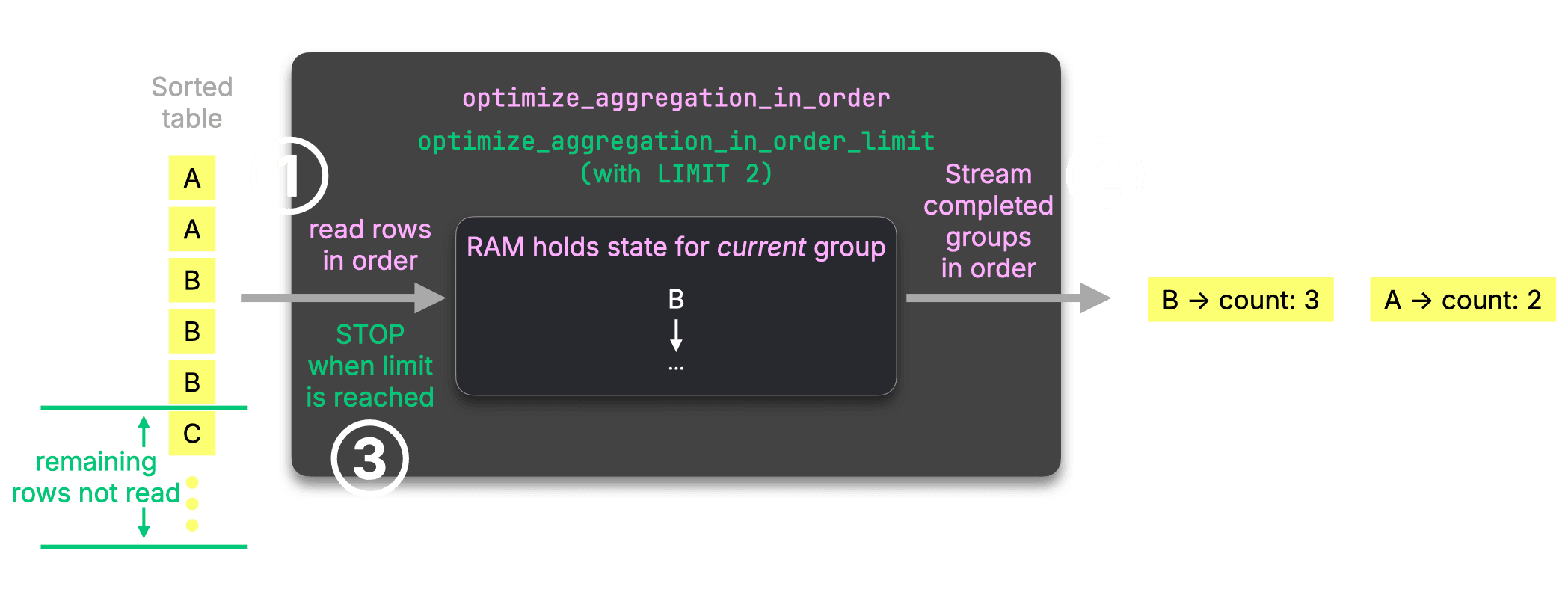
New in 26.7, optimize_aggregation_in_order_limit pushes the LIMIT into that existing ordered-aggregation pipeline. Once N groups have been completed and emitted, ③ ClickHouse stops reading.
Together, the two optimizations turn GROUP BY → ORDER BY → LIMIT into a low-memory, streaming pipeline that can terminate early.
Benchmark: 313× faster and 592× less memory
To evaluate the impact, we created and loaded the TPC-H schema with a scale factor of 100 on an AWS EC2 m6i.8xlarge instance with 32 vCPUs and 128 GiB of RAM.
We benchmark a simple order-summary query. It returns the first 10 orders by order key, together with their number of line items, total quantity, and gross value before discounts and taxes. Because lineitem is sorted by (l_orderkey, l_linenumber), both the GROUP BY and ORDER BY follow the leading sorting-key column - exactly the pattern this optimization targets.
SELECT
    l_orderkey,
    count() AS line_items,
    sum(l_quantity) AS total_quantity,
    sum(l_extendedprice) AS gross_value
FROM lineitem
GROUP BY l_orderkey
ORDER BY l_orderkey
LIMIT 10;First, we disabled both optimize_aggregation_in_order and optimize_aggregation_in_order_limit and ran the query three consecutive times:
10 rows in set. Elapsed: 2.814 sec. Processed 600.04 million rows, 12.00 GB (213.21 million rows/s., 4.26 GB/s.)
Peak memory usage: 17.33 GiB.

10 rows in set. Elapsed: 2.818 sec. Processed 600.04 million rows, 12.00 GB (212.92 million rows/s., 4.26 GB/s.)
Peak memory usage: 17.35 GiB.

10 rows in set. Elapsed: 2.832 sec. Processed 600.04 million rows, 12.00 GB (211.86 million rows/s., 4.24 GB/s.)
Peak memory usage: 17.35 GiB.Next, we enabled both optimizations and repeated the same three-run test:
10 rows in set. Elapsed: 0.009 sec. Processed 1.77 million rows, 35.39 MB (197.78 million rows/s., 3.96 GB/s.)
Peak memory usage: 29.97 MiB.

10 rows in set. Elapsed: 0.010 sec. Processed 1.77 million rows, 35.39 MB (183.80 million rows/s., 3.68 GB/s.)
Peak memory usage: 34.83 MiB.

10 rows in set. Elapsed: 0.009 sec. Processed 1.77 million rows, 35.39 MB (194.19 million rows/s., 3.88 GB/s.)
Peak memory usage: 30.34 MiB.Using the fastest run from each configuration:
| Setting | Runtime | Rows processed | Data processed | Peak memory |
|---|---|---|---|---|
| Both disabled | 2.814 sec | 600.04 million | 12.00 GB | 17.33 GiB |
| Both enabled | 0.009 sec | 1.77 million | 35.39 MB | 29.97 MiB |
| Improvement | 313× faster | 339× fewer | 339× less | 592× less |
Together, the two optimizations deliver a 313× speedup, process 339× fewer rows, and reduce peak memory by 592×.
The right side of a JOIN can now prune the left
Contributed by Shankar Iyer
Each ClickHouse release brings JOIN improvements, and 26.7 comes with three. We start with an optimization that lets the right-hand side guide index pruning on the left: build-side join keys can now eliminate entire probe-side granules before any rows are read.
This targets a common pattern in analytical workloads: selective joins between a large fact table and a much smaller table, or one made small by a selective filter.
Our TPC-H (scale factor 100) example join query has exactly this shape. It calculates revenue from lineitem rows belonging to orders with o_totalprice > 500000:
SELECT
    sum(l.l_extendedprice * (1 - l.l_discount)) AS revenue
FROM lineitem AS l
INNER JOIN orders AS o
    ON l.l_orderkey = o.o_orderkey
WHERE o.o_totalprice > 500000;Before 26.7: Filter rows while reading
For its default parallel hash join algorithm, ClickHouse automatically places the 600-million-row lineitem table on the left, as the probe side, and the filtered orders table on the right, as the build side. ClickHouse also applies runtime filtering:
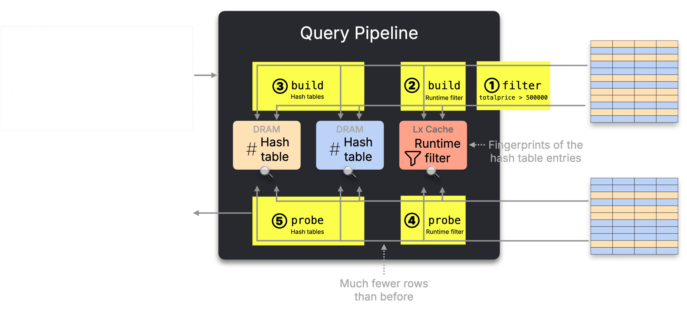
Reading the query pipeline (physical query execution plan) from right to left:
① ClickHouse first applies the o_totalprice > 500000 predicate to orders.
② From the surviving o_orderkey values, it builds a compact runtime filter - a Bloom filter or min/max range.
③ The same filtered orders rows populate the hash tables. The diagram uses max_threads = 2, so two hash tables are built in parallel; normally, max_threads is derived from the number of CPU cores available to the engine.
④ As lineitem rows arrive, their l_orderkey values are checked against the runtime filter. This check is lightweight: the filter is much smaller than the hash tables in step ⑤ and typically remains close to the CPU in L1 or L2 cache.
⑤ Only rows that pass the runtime filter continue to the more expensive hash-table lookup.
This existing runtime filter reduces wasted probe-side work in hash joins by eliminating non-matching probe-side rows before the hash-table lookup. However, by step ④, ClickHouse has already selected the lineitem granules (the smallest processing units in ClickHouse, each covering 8,192 rows by default) and is processing all their rows.
New in 26.7: Skip granules before reading
26.7 inserts one additional runtime phase before the existing row-level filter.
ClickHouse ④ reuses the join keys collected in the runtime filter - either a set of values or a min/max range - for primary-key and skip-index analysis on lineitem. Leveraging the incremental index-evaluation techniques described in our streaming indices post, it skips entire granules that cannot contain matching rows. Those granules are never read:
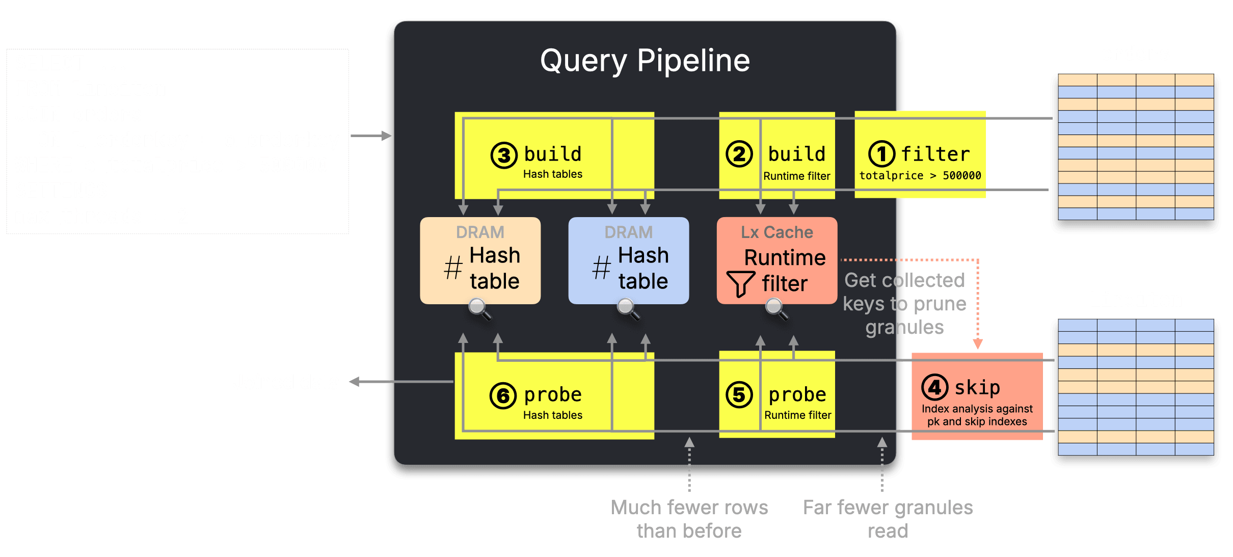
Steps ①–③ remain unchanged: ClickHouse filters the build side, constructs the runtime filter, and populates the hash tables.
The previous probe phases shift by one:
⑤ Rows from the surviving granules are checked against the runtime filter.
⑥ Only rows that pass continue to the more expensive hash-table lookup.
Benchmark: 6.2× faster and 8.8× less memory
To measure the impact, we reused the TPC-H scale-factor-100 dataset and the same AWS EC2 m6i.8xlarge instance as in the previous section, with 32 vCPUs and 128 GiB of RAM.
As a reminder, our example query calculates revenue from lineitem rows belonging to orders with o_totalprice > 500000:
SELECT
    sum(l.l_extendedprice * (1 - l.l_discount)) AS revenue
FROM lineitem AS l
INNER JOIN orders AS o
    ON l.l_orderkey = o.o_orderkey
WHERE o.o_totalprice > 500000;We compared the three relevant join and index optimizations disabled versus enabled. The query condition cache remained disabled in both configurations so that it could not influence the results:
| Setting | Disabled | Enabled |
|---|---|---|
enable_join_runtime_filters | 0 | 1 |
enable_join_runtime_filters_index_analysis | 0 | 1 |
use_skip_indexes_on_data_read | 0 | 1 |
use_query_condition_cache | 0 | 0 |
First, we ran the query three consecutive times with all three optimizations disabled:
1 row in set. Elapsed: 0.600 sec. Processed 750.04 million rows, 13.23 GB (1.25 billion rows/s., 22.03 GB/s.)
Peak memory usage: 19.70 MiB.

1 row in set. Elapsed: 0.597 sec. Processed 750.04 million rows, 13.23 GB (1.26 billion rows/s., 22.14 GB/s.)
Peak memory usage: 29.58 MiB.

1 row in set. Elapsed: 0.599 sec. Processed 750.04 million rows, 13.23 GB (1.25 billion rows/s., 22.10 GB/s.)
Peak memory usage: 25.74 MiB.Next, we enabled all three optimizations and repeated the same three-run test:
1 row in set. Elapsed: 0.099 sec. Processed 162.98 million rows, 1.41 GB (1.65 billion rows/s., 14.29 GB/s.)
Peak memory usage: 3.90 MiB.

1 row in set. Elapsed: 0.097 sec. Processed 162.98 million rows, 1.41 GB (1.68 billion rows/s., 14.51 GB/s.)
Peak memory usage: 6.84 MiB.

1 row in set. Elapsed: 0.097 sec. Processed 162.98 million rows, 1.41 GB (1.67 billion rows/s., 14.48 GB/s.)
Peak memory usage: 3.38 MiB.Using the fastest run from each configuration:
| Setting | Runtime | Rows processed | Data processed | Peak memory |
|---|---|---|---|---|
| All disabled | 0.597 sec | 750.04 million | 13.23 GB | 29.58 MiB |
| All enabled | 0.097 sec | 162.98 million | 1.41 GB | 3.38 MiB |
| Improvement | 6.2× faster | 4.6× fewer | 9.4× less | 8.8× less |
With all three optimizations enabled, the query runs approximately 6.2× faster, processes 4.6× fewer rows and 9.4× less data, and uses 8.8× less peak memory.
Smaller JOIN hash tables with packed row references
Contributed by Harikrishnan Prabakaran
The first JOIN improvement reduces how much probe-side data reaches the join. The second makes the build-side hash tables themselves smaller.
As shown above, ClickHouse inserts right-side rows into in-memory hash tables during the build phase. Each hash-table entry carries a reference to its corresponding row. In 26.7, ClickHouse stores that reference as a compact, 8-byte index-based value for every key type.
As a result, hash-table entries for ALL joins are now as compact as those for ANY joins, reducing memory consumption and improving cache efficiency.
Across joins containing 100–300 million rows, the change produced a median 12% speedup and 15% lower peak memory usage. For INNER joins on UInt64 keys, the improvement reached 21% faster execution and 38% less memory.
DPsub: a third JOIN-ordering algorithm
Contributed by Fisnik Kastrati
The first two JOIN improvements described above optimize efficiency of the the hash join algorithm itself: one reduces probe-side input, while the other shrinks build-side hash tables.
The third works one level higher by automatically choosing how a multi-table query should arrange those joins.
In the first JOIN section above, we saw ClickHouse automatically place the smaller input on the right - the build side - of a two-table parallel hash join. ClickHouse has also supported automatic reordering across larger join graphs for some time.
As described in more detail here, ClickHouse uses column statistics to estimate the sizes of intermediate results and select a good join tree. Until now, it could use exhaustive dpsize search for smaller join graphs or the faster greedy algorithm for larger ones.
26.7 adds a third option: dpsub, which uses dynamic programming over table subsets:
SET query_plan_optimize_join_order_algorithm = 'dpsub';dpsub considers all valid join orders and selects the lowest-cost plan, with lower optimization overhead than dpsize. It also supports non-inner joins.
Algorithms can be chained to provide a fallback:
SET query_plan_optimize_join_order_algorithm = 'dpsub,greedy';ClickHouse tries them in order and falls back when an algorithm cannot handle the query.
Faster vector search with QBit
Vector search finds semantically similar items - such as related documents, products, or images - by comparing their embeddings: high-dimensional numerical representations of the underlying data.
ClickHouse 26.7 introduces several improvements for searching these vectors more efficiently: Int8 support for QBit, strided storage for reading fewer dimensions, randomized Hadamard rotations for better quantization, and quantization codecs for fast two-stage searches. We explore each of them below.
The best way to understand these improvements is to see them in action. Alexey Milovidov built embeddings.info, an interactive, ClickHouse-powered explorer of millions of image embeddings.
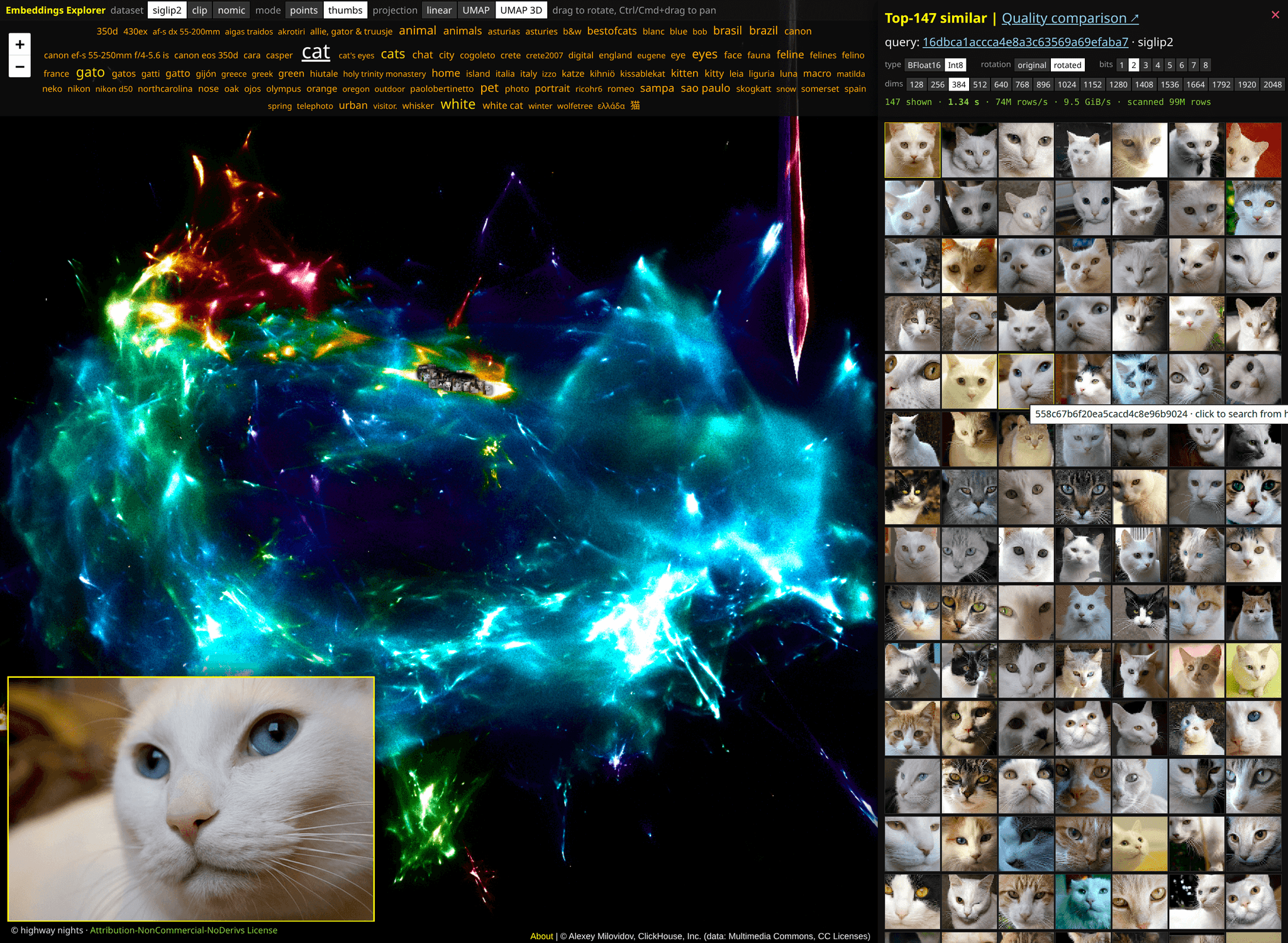
Select an image to find its nearest neighbors, then change the embedding model, numerical representation, rotation, bit precision, or number of dimensions and observe the effect on search speed and quality. The complete implementation and data pipelines are available in the ClickHouse/embeddings repository.
First, a quick QBit refresher. Introduced in ClickHouse 25.10 and production-ready since 26.2, QBit is a data type designed for storing vector embeddings:
CREATE TABLE vectors
(
    id UInt64,
    name String,
    vec QBit(BFloat16, 1536),
    ...
)
ORDER BY (...);Here, QBit(BFloat16, 1536) stores a 1,536-dimensional embedding whose coordinates use the BFloat16 type.
What makes QBit special is that a query can choose how precisely to read those vectors. BFloat16 uses 16 bits per coordinate, and QBit organizes those bits into independently readable planes, from the most to the least significant. A distance query can therefore read only the first N planes:
SELECT id, name
FROM vectors
ORDER BY L2DistanceTransposed(vec, target, 10)
LIMIT 10;The final argument instructs ClickHouse to use the 10 most significant bits out of 16. Reading fewer bits means less I/O and faster distance calculations; reading more provides greater precision and recall.
This matters at scale. One billion 1,536-dimensional BFloat16 vectors contain roughly 3 TB of uncompressed numerical data. Reading 10 rather than all 16 bit planes reduces the vector data read by 37.5%. A query can go further - down to eight or four bits - when speed matters more than perfect recall.
Using fewer bits inevitably loses some information. So how can we preserve more search quality at lower precision?
That brings us to the first QBit improvement in 26.7: Int8 quantization.
QBit: flexible Int8 quantization
Contributed by Alexey Milovidov
Reading fewer bit planes makes vector search faster, but it also discards information. ClickHouse 26.7 adds a more efficient starting point: embeddings can now be quantized to Int8 and stored directly in QBit.
For non-mathematical readers: Quantization represents embedding values with fewer bits, reducing storage and speeding up distance calculations while preserving as much search accuracy as possible.
QBit(Int8, N) preserves QBit’s runtime flexibility. The data is stored as eight bit planes, and each query can choose any precision from a binary representation using one bit to the full eight bits.
ClickHouse’s Int8 quantizer uses 256 non-uniform buckets designed for Gaussian-distributed embedding coordinates. Their boundaries are tuned to minimize the mean-squared error of distance calculations over quantized data. This requires no data scan, distribution estimation, or per-dataset calibration. The specialized quantizeBFloat16ToInt8 and dequantizeInt8ToBFloat16 functions expose this functionality:
CREATE TABLE images
(
    id UInt64,
    emb QBit(Int8, 2048),
    ...
)
ORDER BY (...);

INSERT INTO images
SELECT
    id,
    quantizeBFloat16ToInt8(embedding * sqrt(2048)),
    ...
FROM src;For unit-normalized embeddings, multiplying by the square root of the dimensionality brings the coordinates to the scale expected by the quantizer. Queries can then select their precision at runtime:
SELECT id
FROM images
ORDER BY cosineDistanceTransposedQuantized(emb, target, 4)
LIMIT 10;Here, ClickHouse reads only the four most significant bit planes, half the vector data required by the full eight-bit representation. The distance function interprets the quantized values directly, reconstructing them as part of the calculation. The same stored vectors therefore support everything from 1-bit binary quantization to full 8-bit precision. On the tested datasets, using all eight bits achieved roughly 99–99.5% recall, while lower precisions provide progressively larger I/O savings. Bit precision is only one way to reduce the work. The next improvement lets ClickHouse read fewer vector dimensions as well.
QBit: read fewer dimensions with strided storage
Contributed by Alexey Milovidov
Bit planes let a query control how many bits it reads from each vector coordinate. ClickHouse 26.7 adds a second control: how many dimensions it reads.
An optional third QBit parameter - the stride - divides a vector’s dimensions into independently readable groups
emb QBit(Int8, 1024, 256)This stores the 1,024 dimensions as four groups of 256. Within each group, the eight Int8 bit planes are stored as separate on-disk streams:
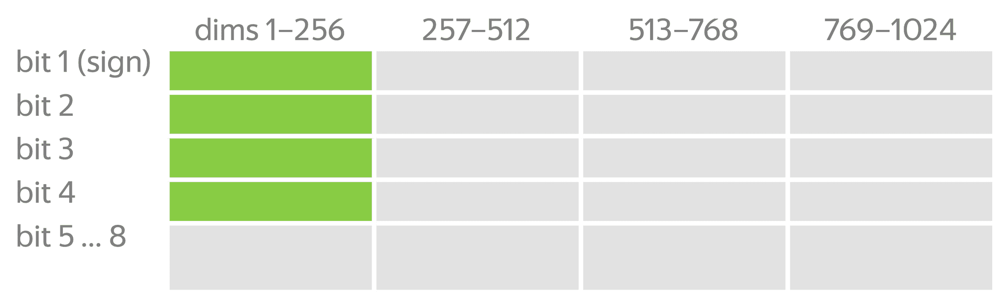
A query can therefore select both its bit precision and the number of dimensions:
...ORDER BY cosineDistanceTransposedQuantized(
    emb,
    target,
    4,     -- read four bit planes
    256    -- read the first 256 dimensions
)This query reads only four bits from the first quarter of the vector: four of the 32 available streams. That is approximately 3% of the equivalent Float32 vector payload.
Strided storage is particularly useful for embeddings trained with Matryoshka Representation Learning. These models arrange information so that prefixes of the vector - such as the first 256 or 512 dimensions - remain useful representations on their own. Queries can therefore trade some recall for substantially less I/O and faster distance calculations without storing several versions of each embedding.
QBit can now vary both the number of bits and the number of dimensions read.
The next improvement focuses on preserving more search quality when those vectors are quantized.
Better quantization with randomized Hadamard rotations
Contributed by Alexey Milovidov
Quantization works best when information is distributed evenly across a vector’s dimensions. Real embeddings are not always so cooperative: some dimensions may carry much larger values or more variation than others, causing low-precision quantization to lose disproportionate amounts of information.
A common solution is to rotate the vector space before quantization. Applying the same orthogonal rotation to every stored vector and query vector preserves their original distances, while spreading information more evenly across dimensions. Quantization can then represent the vectors with less error.
A general random rotation requires an expensive matrix multiplication. Hadamard transforms provide the same kind of mixing much more efficiently. ClickHouse 26.7 introduces randomHadamardTransform as a building block for vector-quantization pipelines:
SELECT randomHadamardTransform(
    [1., 2., 3., 4.]::Array(Float32)
);

-- [0, 2, 1, -5]
-- an orthogonal, norm-preserving rotationThe transformation is deterministic: the same seed produces the same rotation, allowing it to be applied consistently during ingestion and search:
SELECT randomHadamardTransform(v, seed);An optional third argument truncates the transformed vector to a requested number of dimensions:
SELECT randomHadamardTransform(v, seed, 256);This produces a Johnson–Lindenstrauss-style random projection: a smaller representation that approximately preserves distances.
Randomized Hadamard rotations make it possible to build higher-quality quantization pipelines explicitly.
The next improvement packages that work into a codec, so ClickHouse can manage the quantized representation automatically.
Quantization codecs: fast two-stage vector search
Contributed by Shankar Iyer
The previous improvements provide the building blocks for custom quantization pipelines: rotate the vectors, quantize them, store the resulting representation, and call the appropriate distance function.
ClickHouse 26.7 can now manage this automatically through a quantization codec. The codec stores a compact quantized companion alongside the full-precision vectors:
CREATE TABLE vecs
(
    id UInt32,
    v Array(BFloat16) CODEC(Quantized('rabitq', 384)),
    ...
)
ORDER BY (...);Supported methods include int8, one-bit rabitq, two-bit turboquant, mrl, and product quantization (pq). The codec handles the required transformations and maintains both representations.
Quantized codes enable a fast two-stage brute-force search without requiring a vector index:
SET vector_search_use_quantized_codes = 1;

SELECT id
FROM vecs
ORDER BY L2Distance(v, target)
LIMIT 10;In the first stage, ClickHouse scans the much smaller quantized representation and uses approximate distances to select promising candidates. In the second, it reads the full-precision vectors for only those candidates and recalculates their exact distances.
Every vector is still considered, but the expensive full-precision work is restricted to a small shortlist. The quantized first stage can require up to 8× less I/O, while one-bit codes are 16× smaller than the original BFloat16 vectors.
The query itself remains unchanged: enable quantized-code search, and ClickHouse automatically performs the approximate scan followed by full-precision rescoring.
That covers the vector-search improvements in 26.7.
Next, we turn to text search and faster phrase matching.
Position for phrase matching
Contributed by Elmi Ahmadov
Text indexes now store token positions, a feature that’s needed for efficient phrase search. This is an experimental feature at the moment, so you’ll need to enable it by using the allow_experimental_text_index_phrase_search setting.
We’ll test it out using the trusty HackerNews dataset, starting by creating a table that has a text index with phrase search support:
CREATE TABLE hackernews
(
    `id` Int64,
    `deleted` Int64,
    `type` String,
    `by` String,
    `time` DateTime64(9),
    `text` String,
    `dead` Int64,
    `parent` Int64,
    `poll` Int64,
    `kids` Array(Int64),
    `url` String,
    `score` Int64,
    `title` String,
    `parts` Array(Int64),
    `descendants` Int64,
     INDEX idx_text text TYPE text(
       tokenizer = 'splitByNonAlpha', support_phrase_search = 1)

)
ORDER BY time
SETTINGS allow_experimental_text_index_phrase_search = 1;We’ll also create that table (without phrase search support) on ClickHouse 26.6 for comparison. And then we’ll ingest the data:
INSERT INTO hackernews
SELECT *
FROM url('https://datasets-documentation.s3.eu-west-3.amazonaws.com/hackernews/hacknernews.csv.gz', 'CSVWithNames');SELECT count() FROM hackernews WHERE hasPhrase(text, 'Google web search');On 26.6:
┌─count()─┐
│      82 │
└─────────┘

1 row in set. Elapsed: 1.343 sec. Processed 22.67 million rows, 7.57 GB (16.88 million rows/s., 5.64 GB/s.)
Peak memory usage: 247.40 MiB.

┌─count()─┐
│      82 │
└─────────┘

1 row in set. Elapsed: 1.645 sec. Processed 22.67 million rows, 7.57 GB (13.78 million rows/s., 4.60 GB/s.)
Peak memory usage: 280.37 MiB.

┌─count()─┐
│      82 │
└─────────┘

1 row in set. Elapsed: 1.448 sec. Processed 22.67 million rows, 7.57 GB (15.66 million rows/s., 5.23 GB/s.)
Peak memory usage: 282.45 MiB.On 26.7:
┌─count()─┐
│      82 │
└─────────┘

1 row in set. Elapsed: 0.033 sec. Processed 22.67 million rows, 22.67 MB (681.49 million rows/s., 681.49 MB/s.)
Peak memory usage: 42.51 MiB.

1 row in set. Elapsed: 0.034 sec. Processed 22.67 million rows, 22.67 MB (668.31 million rows/s., 668.31 MB/s.)
Peak memory usage: 42.16 MiB.

1 row in set. Elapsed: 0.039 sec. Processed 22.67 million rows, 22.67 MB (588.34 million rows/s., 588.34 MB/s.)
Peak memory usage: 38.66 MiB.The best runtime on 26.6 was 1.343 seconds, compared to 33 milliseconds on 26.7, making 26.7 over 40 times faster.
EXPLAIN ANALYZE
Contributed by Kirill Kopnev
ClickHouse’s EXPLAIN clause family lets you inspect a query at progressively deeper stages of processing: from its parsed abstract syntax tree (AST) and analyzed query tree, through the logical execution plan without yet considering the available execution parallelism (PLAN), to the physical execution plan - the pipeline - showing how those logical plan steps are distributed across parallel processing threads for the available number of CPU cores (PIPELINE).
It can also run index analysis to show which parts and granules primary-key and skip indexes would eliminate, all without executing the complete query.
The EXPLAIN family has continued to grow. In 26.6, hypothetical skip indexes arrived alongside EXPLAIN WHATIF, letting you evaluate an index’s potential effect before materializing it on disk.
In 26.7, EXPLAIN ANALYZE closes the gap between planned and measured execution. It runs every query-processing phase: creating and optimizing the logical execution plan, constructing the physical pipeline, and executing that pipeline. It then discards the result rows and annotates the logical execution-plan tree with measurements collected during actual execution.
Planning time, execution time, and parallelism
EXPLAIN ANALYZE shows the query’s two main phases separately: planning time, covering logical plan creation, plan optimization, and construction of the physical plan (pipeline); and execution time, covering the actual running of that pipeline.
Most notably, EXPLAIN ANALYZE reveals each stage’s observed parallelism - the average number of CPU threads working concurrently compared with the maximum available to that stage. This helps identify potential bottlenecks, particularly stages that run largely serially despite having greater parallel capacity.
Let’s give it a try on the phrase-match query from the previous section:
EXPLAIN ANALYZE
SELECT count()
FROM hackernews
WHERE hasPhrase(text, 'Google web search');┌─explain─────────────────────────────────────────────────────────────────────────────────────┐
│ Query summary: │
│ Time: 29.32 ms (planning 1.74 ms · execution 27.58 ms) │
│ Read: 22.67 million rows, 22.67 MB (822.00 million rows/s., 822.00 MB/s.) │
│ Peak memory: 42.13 MiB │
│ │
│ Output: count() │
│ │
│ Expression ((Project names + Projection)) │
│ │ I/O: rows 1 → 1 · 8 B → 8 B │
│ │ time 1.33 us (0.0%) · parallelism 0.94/1 │
│ └──Aggregating │
│ │ Keys: │
│ │ Aggregates: count() │
│ │ Skip merging: 0 │
│ │ I/O: rows 82 → 1 (1.22%) · 0 B → 8 B │
│ │ Stage (partial aggregation): time 100.30 us (0.4%) · parallelism 0.96/12 │
│ │ Stage (final aggregation): time 2.83 us (0.0%) · parallelism 1.00/1 │
│ └──Expression (Before GROUP BY) │
│ │ I/O: rows 82 → 82 │
│ │ time 16.87 us (0.1%) · parallelism 0.60/12 │
│ └──Filter │
│ │ Filter column: __text_index_idx_text_hasPhrase_df63d4eb06569fbf3c4f7c773f7332ac │
│ │ I/O: rows 22.67 million → 82 (0.00%) · 22.67 MB → 0 B │
│ │ time 2.68 ms (9.7%) · parallelism 2.24/12 │
│ └──ReadFromMergeTree (default.hackernews) │
│ Read type: Default │
│ Parts: 6 | Granules: 3533 │
│ Output: __text_index_idx_text_hasPhrase_df63d4eb06569fbf3c4f7c773f7332ac │
│ Indexes: │
│ PrimaryKey │
│ Condition: true │
│ Parts: 6/6 │
│ Granules: 3533/3533 │
│ Skip │
│ Name: idx_text │
│ Description: text GRANULARITY 100000000 │
│ Condition: (mode: All; tokens: ["Google", "search", "web"]) │
│ Parts: 6/6 │
│ Granules: 3533/3533 │
│ Ranges: 6 │
│ I/O: rows 0 → 22.67 million · 0 B → 22.67 MB │
│ time 27.18 ms (98.6%) · parallelism 11.59/12 │
└─────────────────────────────────────────────────────────────────────────────────────────────┘At the top, the query summary separates the 29.32 ms total runtime into 1.74 ms of planning time and 27.58 ms of execution time. It also reports the total data read, throughput, and peak memory usage.
Below the summary, the annotated plan shows how much data flows through each step, how much execution time it consumes, and how much parallelism its stages achieve.
Reading the plan from bottom to top, ReadFromMergeTree first reads the six selected parts and 3,533 granules from hackernews, producing 22.67 million rows and 22.67 MB. This stage dominates execution at 27.18 ms, or 98.6% of execution time, while averaging 11.59 of 12 available CPU threads, almost full parallelism.
The Filter step then applies hasPhrase(text, 'Google web search'), reducing those 22.67 million candidate rows to just 82 matches. It takes 2.68 ms, or 9.7% of execution time, with an average parallelism of 2.24 out of 12 CPU threads.
Finally, the aggregation turns the 82 matching rows into the single count() result. Its partial stage averages roughly one thread, while the final aggregation is single-threaded. With so little data remaining, there is no useful work to distribute further.
At a glance, we can see where the query spends its time, how data is reduced as it moves through the pipeline, and how effectively each stage uses the available CPU parallelism.
Remote and RemoteSecure engines
Contributed by Alexey Milovidov
Data federation is a core ClickHouse capability. The query engine can read and join data directly from more than 60 external systems and over 100 formats without first ingesting it into ClickHouse.
This can be done via table functions, which expose a remote data source as a table that can be used in SELECT - and, for many sources, INSERT - just like a local ClickHouse table. Many table functions also have corresponding table engines, allowing the connection to be defined once instead of repeated in every query.
The long-standing remote and remoteSecure table functions provide ClickHouse-to-ClickHouse federation: one cluster can read from and write to tables hosted by another cluster. ClickHouse 26.7 adds dedicated Remote and RemoteSecure table engines for defining these connections persistently.
Persistent remote tables simplify multi-region analytics, centralized reporting across isolated deployments, and migrations or backfills with INSERT SELECT. They are especially useful in ClickHouse Cloud, where RemoteSecure can expose a table from another service or region under a regular local table name.
Example
Suppose the prod server hosts an events table in its default database. We can expose it under a persistent local table name:
CREATE TABLE events_on_prod
ENGINE = Remote('prod:9000', default, events);No column list is required: ClickHouse infers the structure from the remote table. The resulting table is a persistent link. Reads and writes are forwarded to prod:
SELECT count()
FROM events_on_prod;

INSERT INTO events_on_prod
SELECT *
FROM local_events;RemoteSecure provides the same capability over TLS. Both engines also support cluster-style address patterns such as host{1..3}:9000, or host{1..3}:9440 over TLS.
Unification of URL
Contributed by Alexey Milovidov
The url table function and URL table engine now dispatch to the right backend based on the URL scheme.
It works for file paths, S3, GCS, Azure, and HDFS, and HTTP will continue to work as before.
Below is an example of how we can now query the Amazon reviews dataset from its S3 bucket:
SELECT count(), avg(star_rating)
FROM url('s3://datasets-documentation/amazon_reviews/amazon_reviews_2015.snappy.parquet');┌──count()─┬──avg(star_rating)─┐
│ 41905631 │ 4.249571829618793 │
└──────────┴───────────────────┘For backends that need credentials, these can be passed through as extra parameters or provided as environment variables.
For example, to query S3, we can pass credentials through like this:
SELECT count()
FROM url(
  's3://not/public/file.parquet',
  '',
  '',
  ''
);Or (when using clickhouse-local), provide them as environment variables:
export AWS_ACCESS_KEY_ID=""
export AWS_SECRET_ACCESS_KEY=""
export AWS_SESSION_TOKEN=""SELECT count()
FROM url(
's3://not/public/file.parquet',
);DateTime64: Years 0 to 9999
Contributed by Alexey Milovidov
Before ClickHouse 26.7, the DateTime64 type supported values from 1900 to 2299. As of the 26.7 release, it now supports values from 0000-01-01 to 9999-12-31.
Let’s have a look at how this works with help from a small dataset of historic and projected events:
SELECT *
FROM s3('s3://public-pme/26.7/history_events.parquet')
LIMIT 10;┌─event────────────────────────────────────────────┬─happened────────────────┬─category────┐
│ Eruption of Mount Vesuvius buries Pompeii │ 0079-08-24 13:00:00.000 │ disaster │
│ Roman Emperor Hadrian begins the wall in Britain │ 0122-01-01 00:00:00.000 │ politics │
│ Diocletian splits the Roman Empire │ 0285-01-01 00:00:00.000 │ politics │
│ Council of Nicaea convenes │ 0325-05-20 00:00:00.000 │ religion │
│ Fall of the Western Roman Empire │ 0476-09-04 00:00:00.000 │ politics │
│ Justinian's Corpus Juris Civilis published │ 0534-01-01 00:00:00.000 │ law │
│ The Hijra: Muhammad travels to Medina │ 0622-09-24 00:00:00.000 │ religion │
│ Coronation of Charlemagne as Holy Roman Emperor │ 0800-12-25 12:00:00.000 │ politics │
│ Leif Erikson reaches North America │ 1000-01-01 00:00:00.000 │ exploration │
│ Norman conquest at the Battle of Hastings │ 1066-10-14 09:00:00.000 │ military │
└──────────────────────────────────────────────────┴─────────────────────────┴─────────────┘Let’s create a table:
CREATE TABLE history
(
    event    String,
    happened DateTime64(3),
    category LowCardinality(String)
)
ENGINE = MergeTree
ORDER BY happened;And then ingest the data:
INSERT INTO history
SELECT *
FROM s3('s3://public-pme/26.7/history_events.parquet');We can then work out how long it’s been since events happened:
SELECT event, age('year', happened, now()) AS years_ago
FROM history
WHERE category != 'future'
ORDER BY years_ago DESC
LIMIT 10;┌─event────────────────────────────────────────────┬─years_ago─┐
│ Eruption of Mount Vesuvius buries Pompeii │ 1946 │
│ Roman Emperor Hadrian begins the wall in Britain │ 1904 │
│ Diocletian splits the Roman Empire │ 1742 │
│ Council of Nicaea convenes │ 1702 │
│ Fall of the Western Roman Empire │ 1550 │
│ Justinian's Corpus Juris Civilis published │ 1492 │
│ The Hijra: Muhammad travels to Medina │ 1403 │
│ Coronation of Charlemagne as Holy Roman Emperor │ 1225 │
│ Leif Erikson reaches North America │ 1027 │
│ Norman conquest at the Battle of Hastings │ 960 │
└──────────────────────────────────────────────────┴───────────We could also compute one millennium into the future from a date, which wasn’t previously possible if the resulting date exceeded 2299:
SELECT event, happened, happened + INTERVAL 1000 YEAR AS one_millennium_later
FROM history
WHERE happened > '1300-01-01'
ORDER BY happened
LIMIT 5;┌─event──────────────────────────────────┬────────────────happened─┬────one_millennium_later─┐
│ The Black Death reaches Europe │ 1347-10-01 00:00:00.000 │ 2347-10-01 00:00:00.000 │
│ Gutenberg completes the printing press │ 1440-01-01 00:00:00.000 │ 2440-01-01 00:00:00.000 │
│ Fall of Constantinople to the Ottomans │ 1453-05-29 06:00:00.000 │ 2453-05-29 06:00:00.000 │
│ Columbus reaches the Americas │ 1492-10-12 06:00:00.000 │ 2492-10-12 06:00:00.000 │
│ Vasco da Gama reaches India by sea │ 1498-05-20 00:00:00.000 │ 2498-05-20 00:00:00.000 │
└────────────────────────────────────────┴─────────────────────────┴─────────────────────────┘groupFormat
Contributed by Yang Hu
groupFormat is an aggregate function that formats each group’s rows with any output format, returning the result as a string.
It’s a useful function for grouping data to send to LLMs or webhooks, as well as for reports.
The following query groups the history dataset by century and returns JSON-formatted event names and years for each group:
SELECT intDiv(toYear(happened), 100) + 1  AS century,
       groupFormat('JSONEachRow')(event, toYear(happened))
FROM history
GROUP BY century HAVING length(groupArray(happened)) > 1
ORDER BY century
LIMIT 5;┌─century─┬─groupFormat('JSONEachRow')(event, toYear(happened))────────────────┐
│ 11 │ {"c1":"Leif Erikson reaches North America","c2":1000} ↴│
│ │↳{"c1":"Norman conquest at the Battle of Hastings","c2":1066} ↴│
│ │↳{"c1":"First Crusade captures Jerusalem","c2":1099} ↴│
│ 13 │ {"c1":"Signing of the Magna Carta","c2":1215} ↴│
│ │↳{"c1":"Marco Polo departs for Asia","c2":1271} ↴│
│ 15 │ {"c1":"Gutenberg completes the printing press","c2":1440} ↴│
│ │↳{"c1":"Fall of Constantinople to the Ottomans","c2":1453} ↴│
│ │↳{"c1":"Columbus reaches the Americas","c2":1492} ↴│
│ │↳{"c1":"Vasco da Gama reaches India by sea","c2":1498} ↴│
│ 16 │ {"c1":"Luther posts the Ninety-five Theses","c2":1517} ↴│
│ │↳{"c1":"Magellan's expedition circumnavigates the globe","c2":1522}↴│
│ │↳{"c1":"Copernicus publishes On the Revolutions","c2":1543} ↴│
│ │↳{"c1":"Defeat of the Spanish Armada","c2":1588} ↴│
│ 17 │ {"c1":"Galileo observes the moons of Jupiter","c2":1610} ↴│
│ │↳{"c1":"The Mayflower reaches Plymouth","c2":1620} ↴│
│ │↳{"c1":"Newton publishes the Principia","c2":1687} ↴│
└─────────┴────────────────────────────────────────────────────────────────────┘Drivers for executable UDFs
Contributed by Daniil Timižev and Alexey Milovidov
ClickHouse already supports executable user-defined functions, but creating one previously required two separate steps outside SQL: preparing the executable itself and writing the ClickHouse configuration that describes how to run it.
ClickHouse 26.7 introduces experimental drivers for executable UDFs. Once a driver for a programming language or toolchain is configured on the server, users can write the complete UDF in C, Rust, Python, or any other supported language directly inside a standard SQL CREATE FUNCTION statement. That statement is all the user needs: there is no separate source file, compilation step, executable deployment, or executable-UDF configuration.
The driver handles everything else. It takes the function signature and embedded source code from CREATE FUNCTION, compiles, interprets, or otherwise processes it, and produces the executable and configuration that ClickHouse already knows how to load and run.
A driver is a server-side recipe defined in XML or YAML. It declares:
- The name exposed through
CREATE FUNCTION ... ENGINE. - The command that creates the executable UDF.
- An optional cleanup command.
- Optional validated arguments for configuring the driver from SQL.
- Optional environment variables supplied to its commands.
The language accepted inside CREATE FUNCTION is determined by the selected driver.
The proof-of-concept GVisorC driver included in the PR is specifically built for C: its creation script accepts a C function body, wraps and compiles it, and produces an executable UDF:
<clickhouse>
<driver>
<name>GVisorC</name>
<create_command>
../user_defined_executable_function_drivers/gvisor_c_create.sh
</create_command>
<drop_command>
../user_defined_executable_function_drivers/gvisor_c_drop.sh
</drop_command>
<env>
<CLICKHOUSE_C_DRIVER_MEMORY>256m</CLICKHOUSE_C_DRIVER_MEMORY>
<CLICKHOUSE_C_DRIVER_CPUS>1.0</CLICKHOUSE_C_DRIVER_CPUS>
<CLICKHOUSE_C_DRIVER_GVISOR_BINARY>runsc</CLICKHOUSE_C_DRIVER_GVISOR_BINARY>
</env>
</driver>
</clickhouse>The referenced gvisor_c_create.sh and gvisor_c_drop.sh scripts are included in the PR as part of the proof-of-concept driver. They implement the creation and cleanup steps referenced by the configuration.
BecauseENGINE = GVisorC() selects this C-specific driver, the AS clause can contain the complete C function body directly:
CREATE FUNCTION add
ARGUMENTS (x UInt8, y UInt8)
RETURNS Int64
ENGINE = GVisorC()
AS 'return (int64_t) x + (int64_t) y;';

SELECT add(40, 2);42The complete creation flow looks like this:
ENGINE = GVisorC()selects the driver whose configured name isGVisorC.- ClickHouse invokes its
create_command, passing the function name, return type, argument signature, and any declared engine arguments. The function body is sent through standard input, together with the configured environment. - The
GVisorCdriver generates the surrounding executable-UDF code, compiles it, and returns the standard executable-UDF configuration. - ClickHouse stores and loads that configuration through its existing executable-UDF machinery.
- The original definition is persisted as an
ATTACH FUNCTIONstatement, so the function survives server restarts. DROP FUNCTIONinvokes the optionaldrop_commandand removes the generated configuration and working files.
The GVisorC example compiles C function bodies and runs the generated executables inside gVisor sandboxes. The PR also contains DockerC and UnsafeC examples, but the driver mechanism itself is language- and toolchain-independent: deployments can define drivers for Python, Rust, C, or other environments.
That is why these components are called drivers: they translate a compact, language-specific function definition into the executable and configuration that ClickHouse already knows how to run. Drivers are how ClickHouse makes executable UDFs directly accessible to users.
Note that the included C drivers are proofs of concept and are not installed by ClickHouse packages. See the implementation PR and the complete GVisorC driver configuration.
The built-in Web UI grows into a real SQL workspace
Contributed by Alexey Milovidov
ClickHouse 26.7 gives its open-source, embedded Web UI (/play endpoint) a major feature boost. What began as a convenient browser-based query console now feels like a complete SQL workspace:
- Work on multiple queries in tabs. Titles, parameters, and small result snapshots persist across reloads, with state integrated into browser history and the URL.
- Navigate databases, tables, and columns from the improved database panel, including data types, compressed and uncompressed sizes, and compression ratios.
- Write queries faster with schema-aware autocompletion, keyboard navigation, matching-identifier and parenthesis highlighting, inline syntax errors, and improved indentation.
- Explore results using per-column bar, heatmap, or categorical coloring, and pin important columns while scrolling wide tables.
- Run parameterized queries and watch results update progressively while a query is executing.
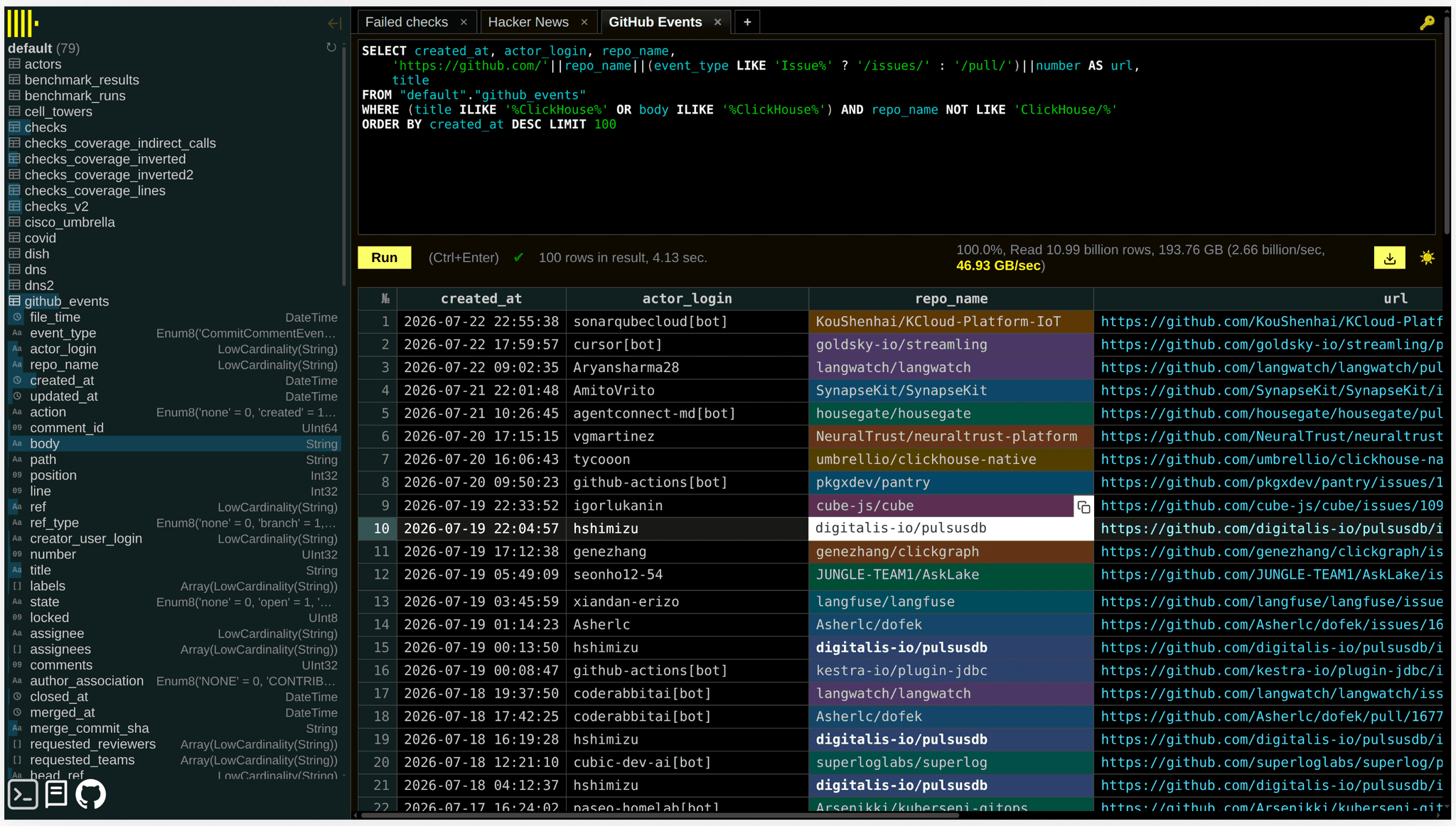
That is a lot to describe in a feature list, and the result is much better seen in action. The interface is fast, polished, and genuinely enjoyable to use. See for yourself - the video below jumps directly to Alexey’s demo:
Instant, version-matched reference docs
Contributed by Alexey Milovidov
The embedded Web UI now has a natural companion: every ClickHouse server exposes searchable reference documentation at /docs.
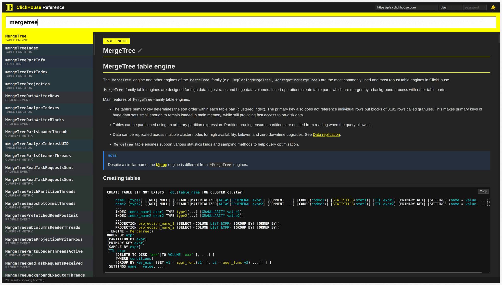
The page searches system.documentation for functions, settings, table engines, data types, formats, and more, then renders complete reference pages with syntax highlighting, mathematical formulas, and cross-links. Because everything comes from the server itself, it works without internet access and always matches the ClickHouse version you are running.
Under the hood, search is simply a query against a ClickHouse system table, so results appear instantly.
See it in action - the video below starts directly at Alexey’s demo:
We’ll close with two more kinds of speed: faster regular-expression processing and a substantially faster ClickHouse on macOS.
Regular expressions, compiled to native code
Contributed by Alexey Milovidov
ClickHouse uses the fastest libraries it can find. For regular expressions, that starts with RE2, created by Russ Cox. ClickHouse also uses Vectorscan, which accelerates suitable patterns with SIMD.
But even that was not fast enough.
In 26.7, ClickHouse adds its own JIT-compiled regexp engine. For supported patterns, it uses LLVM to compile the regular expression on the fly into native machine code optimized for the CPU running the query:
SELECT count()
FROM logs
WHERE match(line, '^[a-z]+[0-9]+@example[0-9]+\\.com$');The new engine accelerates match, extract, extractAll, replaceRegexpOne, replaceRegexpAll, and LIKE. It is enabled by default through compile_regular_expressions; unsupported patterns transparently fall back to the alternative libraries.
There is nothing to rewrite or configure: upgrade to 26.7, and existing regexp queries automatically take the faster path whenever possible.
In a test running match() over 20 million strings, execution time dropped from 2.7 seconds to 1.1 seconds - about 2.5× faster.
ClickHouse gets faster on macOS
Contributed by Alexey Milovidov and Raúl Marín
ClickHouse 26.7 also closes several performance and feature gaps on macOS:
-
jemallocnow purges dirty pages in a background thread instead of eagerly, matching its behavior on Linux. Allocation-heavy workloads such as recursive CTEs run approximately 2× faster. -
Per-CPU
jemallocarenas and allocation profiling are now enabled. -
Asynchronous reads from remote replicas now work through an
epollcompatibility layer backed bykqueue, allowing distributed queries to read from shards concurrently instead of serially. -
SSD cache dictionaries and the
FileLogengine now work on macOS. -
STREAMqueries are now supported.
For developers running ClickHouse locally on Apple hardware, 26.7 is both faster and more complete.