Get started with ClickHouse Cloud today and receive $300 in credits. To learn more about our volume-based discounts, contact us or visit our pricing page.
This blog post is part of a series:
- Join Types supported in ClickHouse
- ClickHouse Joins Under the Hood - Full Sorting Merge Join, Partial Merge Join
- ClickHouse Joins Under the Hood - Direct Join
- Choosing the Right Join Algorithm
In our previous post, we reviewed the SQL JOIN types that are available in ClickHouse. As a reminder: ClickHouse comes with full SQL Join Support.
In this post, we’ll start the exploration the internals of join execution in ClickHouse, so that you can optimize joins for queries used by your applications. Here, you’ll see how ClickHouse integrates these classical join algorithms to its query pipeline in order to execute the join types as fast as possible.
Query Pipeline
ClickHouse is designed to be fast. Queries in ClickHouse are processed in a highly parallel fashion, taking all the necessary resources available on the current server and in many cases, utilizing hardware up to its theoretical limits. The more CPU cores and main memory a server has the more performance gains from parallel execution a query will have.
The Query Pipeline determines the level of parallelism for each query execution stage.
The following diagram shows how the ClickHouse Query Pipeline processes a query on a server with 4 CPU cores:
 The table data queried is dynamically spread among 4 separate and parallel stream stages, which stream the data block-wise into ClickHouse. Because the server has 4 CPU cores, most query processing stages from the query pipeline are executed by 4 threads in parallel.
The amount of threads utilized is dependent on the max_threads setting, which by default is set to the number of CPU cores that ClickHouse sees on the machine it is running on.
For all queries -- joins included -- the query pipeline ensures that the table data is processed in a highly parallel and scalable manner.
Join algorithms under the hood
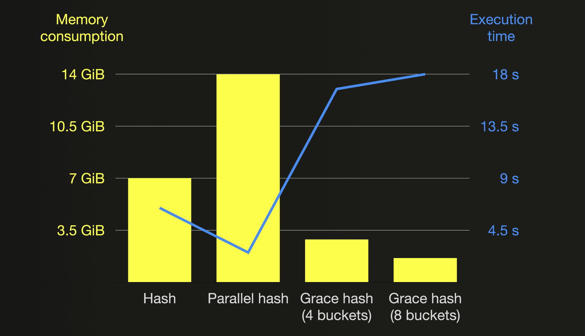
To ensure maximum utilization of resources, 6 different join algorithms have been developed for ClickHouse. These algorithms dictate the manner in which a join query is planned and executed. ClickHouse can be configured to adaptively choose and dynamically change the join algorithm to use at runtime. Depending on resource availability and usage. However, ClickHouse also allows users to specify the desired join algorithm themselves. This chart gives an overview of these algorithms based on their relative memory consumption and execution time:

This blog post will describe and compare in detail the three ClickHouse join algorithms from the chart above that are based on in-memory hash tables:
We will explore in this post how the Hash join algorithm is fast and most generic. The Parallel hash join algorithm can be faster with large right-hand side tables but requires more memory. Both the hash join and parallel hash join are memory-bound. Whereas the Grace hash join is a non-memory bound version that spills data temporarily to disk. Grace hash join doesn’t require any sorting of the data and therefore overcomes some of the performance challenges of other join algorithms that spill data to disk like the (partial) merge join algorithm (we will cover this in the second part).
In the next post, we will have a look at the two algorithms from the chart above that are based on external sorting:
We keep the best for the end and will finish our exploration of the ClickHouse join algorithms in another post where we will describe ClickHouse’s fastest join algorithm from the chart above:
Test Data and Resources
For all example queries, we are going to use two of the tables from the normalized IMDB dataset that we introduced in the previous post:

In order to have sizable data to test with, we generated large versions of these tables in a new database imdb_large.
This query lists the number of rows and amount of uncompressed data in the example tables:
SELECT
    table,
    formatReadableQuantity(sum(rows)) AS rows,
    formatReadableSize(sum(data_uncompressed_bytes)) AS data_uncompressed
FROM system.parts
WHERE (database = 'imdb_large') AND active
GROUP BY table
ORDER BY table ASC;

┌─table──┬─rows───────────┬─data_uncompressed─┐
│ actors │ 1.00 million   │ 21.81 MiB         │
│ roles  │ 100.00 million │ 2.63 GiB          │
└────────┴────────────────┴───────────────────┘
For all visualizations, in order to keep them succinct and readable, we artificially limit the level of parallelism used within the ClickHouse query pipeline with the setting max_threads = 2.
However, for all example query runs, we use the default setting of max_threads.
As mentioned above, by default, max_threads is set to the number of CPU cores that ClickHouse sees on the machine it is running on. These examples use a ClickHouse Cloud service, where a single node has 30 CPU cores:
SELECT getSetting('max_threads');

┌─getSetting('max_threads')─┐
│                        30 │
└───────────────────────────┘
Now let’s start exploring ClickHouse join algorithms. We begin with the most generic one, the hash join algorithm.
Hash join
Description
An in-memory hash table can serve 250 million totally random requests per second (and more than a billion if it fits in the CPU cache). This very fast lookup capability makes the in-memory hash table a natural general choice in ClickHouse for implementing joins when it is not possible or feasible to take advantage of table sorting.
The hash join algorithm is the most generic of the available join implementations in ClickHouse. We illustrate the hash join algorithm integrated into the ClickHouse query pipeline below:
 We can see that:
① All data from the right-hand side table is streamed (in parallel by 2 threads because max_threads = 2) into the memory, and then ClickHouse fills an in-memory hash table with this data.
② Data from the left-hand side table is streamed (in parallel by 2 threads because max_threads = 2) and ③ joined by doing lookups into the hash table.
Note that because ClickHouse takes the right-hand side table and creates a hash table for it in RAM, it is more memory efficient to place the smaller table on the right-hand side of the JOIN. We will demonstrate that below.
Also note that the Hash table is a key data structure in ClickHouse. Based on each specific query and, for join queries specifically, based on join key column types and join strictness, ClickHouse automatically chooses one of 30+ variations.
Supported join types
All join types and strictness settings are supported. In addition, currently, only the hash join supports multiple join keys that are combined with OR in the ON clause.
For readers wanting to dive even deeper, the source code contains a very detailed description of how these types and settings are implemented by the hash join algorithm.
Examples
We demonstrate the hash join algorithm with two query runs.
Smaller table on the right-hand side:
SELECT *
FROM roles AS r
JOIN actors AS a ON r.actor_id = a.id
FORMAT `Null`
SETTINGS join_algorithm = 'hash';

0 rows in set. Elapsed: 0.817 sec. Processed 101.00 million rows, 3.67 GB (123.57 million rows/s., 4.49 GB/s.)
Larger table on the right-hand side:
SELECT *
FROM actors AS a
JOIN roles AS r ON a.id = r.actor_id
FORMAT `Null`
SETTINGS join_algorithm = 'hash';

0 rows in set. Elapsed: 5.063 sec. Processed 101.00 million rows, 3.67 GB (19.95 million rows/s., 724.03 MB/s.)
We can query the query_log system table in order to check runtime statistics for the last two query runs:
SELECT
    query,
    formatReadableTimeDelta(query_duration_ms / 1000) AS query_duration,
    formatReadableSize(memory_usage) AS memory_usage,
    formatReadableQuantity(read_rows) AS read_rows,
    formatReadableSize(read_bytes) AS read_data
FROM clusterAllReplicas(default, system.query_log)
WHERE (type = 'QueryFinish') AND hasAll(tables, ['imdb_large.actors', 'imdb_large.roles'])
ORDER BY initial_query_start_time DESC
LIMIT 2
FORMAT Vertical;

Row 1:
──────
query:          SELECT *
                FROM actors AS a
                JOIN roles AS r ON a.id = r.actor_id
                FORMAT `Null`
                SETTINGS join_algorithm = 'hash'
query_duration: 5 seconds
memory_usage:   8.95 GiB
read_rows:      101.00 million
read_data:      3.41 GiB

Row 2:
──────
query:          SELECT *
                FROM roles AS r
                JOIN actors AS a ON r.actor_id = a.id
                FORMAT `Null`
                SETTINGS join_algorithm = 'hash'
query_duration: 0 seconds
memory_usage:   716.44 MiB
read_rows:      101.00 million
read_data:      3.41 GiB
As expected, the join query with the smaller actors table on the right-hand side consumes significantly less memory than the join query with the larger roles table on the right-hand side.
Note that the indicated peak memory usages of 8.95 GiB and 716.44 MiB, are larger than the uncompressed sizes of 2.63 GiB and 21.81 MiB for the respective right-hand side tables for the two query runs. The reason for this is that the hash table size is initially chosen and dynamically increased based on the types of the join key columns and in multiples of a specific internal hash table buffer size. The memory_usage metric counts the overall memory reserved for the hash table, though it may not be completely filled.
For the execution of both queries, ClickHouse reads the same amount of total rows (and data): 100 million rows from the roles table + 1 million rows from the actors table. However, the join query with the larger roles table on the right-hand side is five times slower. This is because the default hash join is not thread-safe for inserting the right table's rows into the hash table. Therefore the fill stage for the hash table runs in a single thread. We can double-check this by introspecting the actual query pipeline.
Query pipeline
We can introspect the ClickHouse query pipeline for a hash join query by using the ClickHouse command line client (quick install instructions are here). We use the EXPLAIN statement for printing a graph of the query pipeline described in the DOT graph description language, and use Graphviz dot for rendering the graph in pdf format:
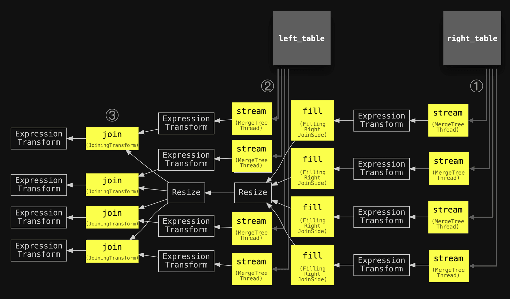
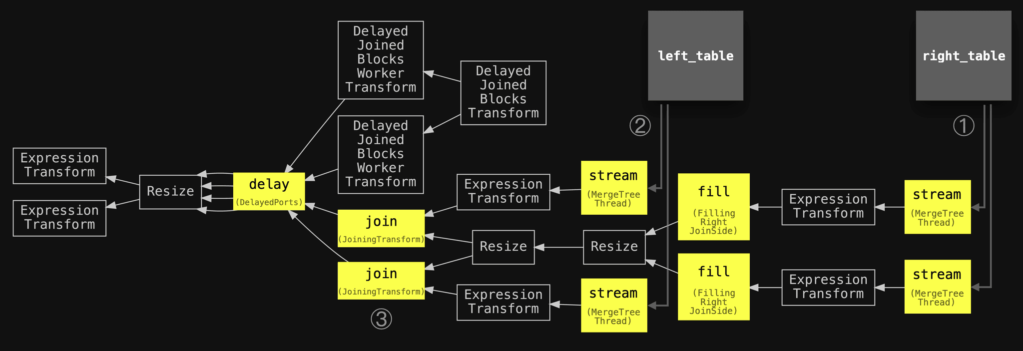
We have annotated the pipeline with the same circled numbers used in the abstract diagram above, slightly simplified the names of the main stages, and added the two joined tables in order to align the two diagrams:./clickhouse client --host ekyyw56ard.us-west-2.aws.clickhouse.cloud --secure --port 9440 --password --database=imdb_large --query " EXPLAIN pipeline graph=1, compact=0 SELECT * FROM actors a JOIN roles r ON a.id = r.actor_id SETTINGS max_threads = 2, join_algorithm = 'hash';" | dot -Tpdf > pipeline.pdf
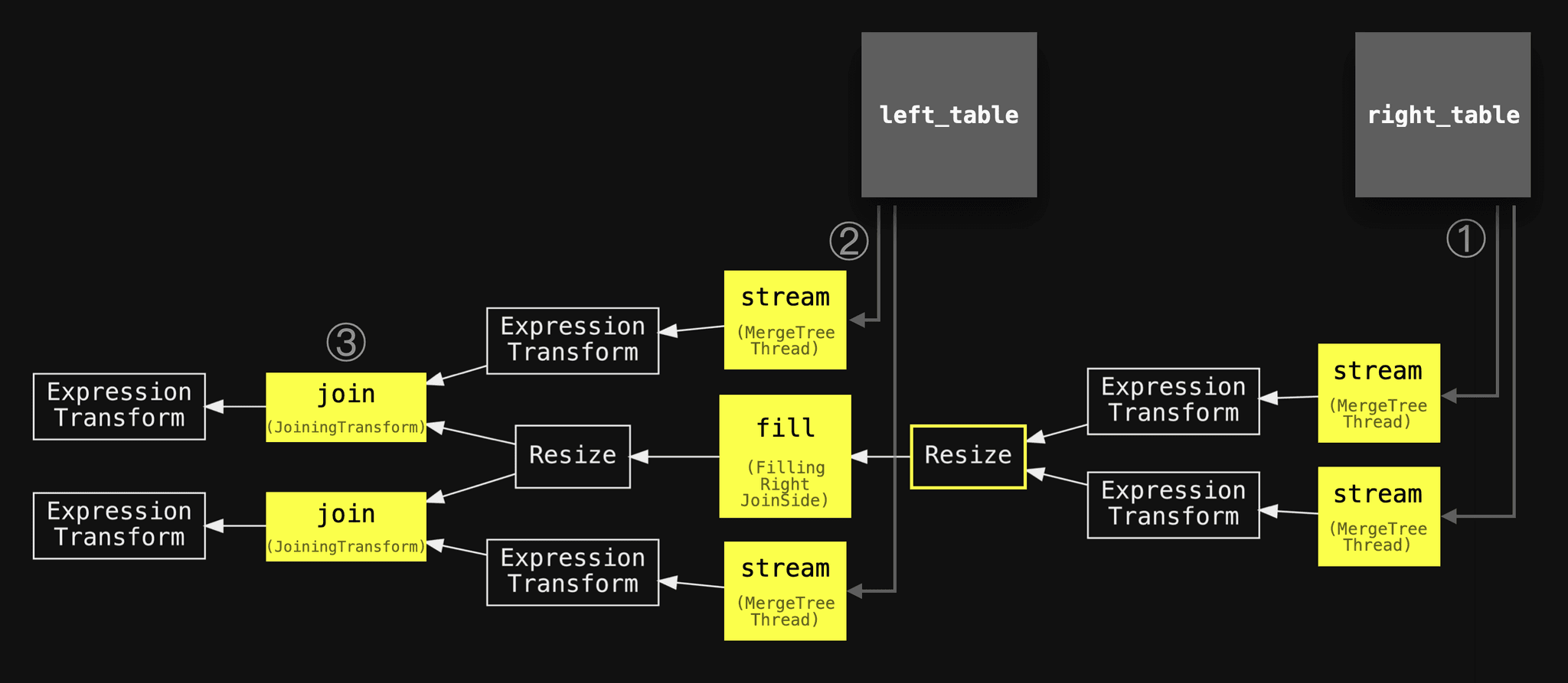
We can see the query pipeline ① starts with two parallel stream stages (because max_threads is set to 2) for streaming the data from the right-hand side table, followed by a single fill stage for filling the hash table. Two additional parallel stream stages ② and two parallel join stages ③ are used for streaming and joining the data from the left-hand side table.
As mentioned above, the default hash join algorithm is not thread-safe for inserting the right-hand side table's rows into the hash table. Therefore a resize stage is used in the pipeline above for reducing the two threads streaming the data from the right-hand side table into a single-threaded fill stage. This can become a bottleneck for the query runtime. If the right-hand side table is large - see our two query runs above where the query with the large roles table on the right-hand side of the join was five times slower.
However, since ClickHouse version 22.7 the process of building the hash table from the right-hand side table can be significantly sped up for large tables by using the parallel hash algorithm.
Parallel hash join
Description
The parallel hash join algorithm is a variation of a hash join that splits the input data to build several hash tables concurrently in order to speed up the join at the expense of higher memory overhead. We sketch this algorithm's query pipeline below:
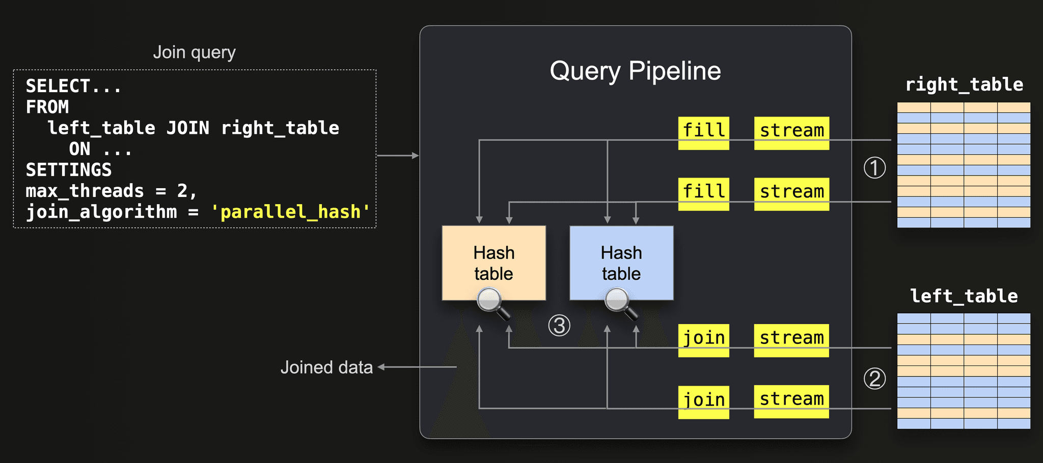
The diagram above shows that:
① All data from the right table is streamed (in parallel by 2 threads because max_threads = 2) into the memory. The data is streamed block-wise. The rows from each streamed block are split into 2 buckets ( max_threads = 2) by applying a hash function to the join keys of every row. We sketch this with the orange and blue colors in the diagram above. In parallel, one in-memory hash table is filled per bucket using a single thread. Note that the hash function for splitting the rows into buckets is different from the one that is used in the hash tables internally.
② Data from the left table is streamed (in parallel by 2 threads because max_threads = 2), and the same ‘bucket hash function’ from step ① is applied to the join keys of each row for determining the corresponding hash table and the rows are ③ joined by doing lookups into the corresponding hash table.
Note that the max_threads setting determines the number of concurrent hash tables. We will demonstrate that later by introspecting concrete query pipelines.
Supported join types
INNER and LEFT join types and all strictness settings except ASOF are supported.
Examples
We will now compare the runtimes and peak memory consumption of the hash and parallel hash algorithms for the same query.
Hash join with a larger table on the right-hand side:
SELECT *
FROM actors AS a
JOIN roles AS r ON a.id = r.actor_id
FORMAT `Null`
SETTINGS join_algorithm = 'hash';

0 rows in set. Elapsed: 5.385 sec. Processed 101.00 million rows, 3.67 GB (18.76 million rows/s., 680.77 MB/s.)
Parallel hash join with larger table on the right-hand side:
SELECT *
FROM actors AS a
JOIN roles AS r ON a.id = r.actor_id
FORMAT `Null`
SETTINGS join_algorithm = 'parallel_hash';

0 rows in set. Elapsed: 2.639 sec. Processed 101.00 million rows, 3.67 GB (38.28 million rows/s., 1.39 GB/s.)
We check runtime statistics for the last two query runs:
SELECT
    query,
    formatReadableTimeDelta(query_duration_ms / 1000) AS query_duration,
    formatReadableSize(memory_usage) AS memory_usage,
    formatReadableQuantity(read_rows) AS read_rows,
    formatReadableSize(read_bytes) AS read_data
FROM clusterAllReplicas(default, system.query_log)
WHERE (type = 'QueryFinish') AND hasAll(tables, ['imdb_large.actors', 'imdb_large.roles'])
ORDER BY initial_query_start_time DESC
LIMIT 2
FORMAT Vertical;

Row 1:
──────
query:          SELECT *
                FROM actors AS a
                JOIN roles AS r ON a.id = r.actor_id
                FORMAT `Null`
                SETTINGS join_algorithm = 'parallel_hash'
query_duration: 2 seconds
memory_usage:   18.29 GiB
read_rows:      101.00 million
read_data:      3.41 GiB

Row 2:
──────
query:          SELECT *
                FROM actors AS a
                JOIN roles AS r ON a.id = r.actor_id
                FORMAT `Null`
                SETTINGS join_algorithm = 'hash'
query_duration: 5 seconds
memory_usage:   8.86 GiB
read_rows:      101.00 million
read_data:      3.41 GiB
The parallel hash join was roughly 100% faster than the standard hash join, but had more than twice the peak memory consumption, although the amount of rows and data read, as well as the size of the right-hand side table is the same for both queries.
The reason for this much higher memory consumption is that the query was run on a node with 30 CPU cores and, therefore, with a max_threads setting of 30. This means that, as we will demonstrate below, 30 concurrent hash tables were used. As mentioned before, the size for each hash table is initially chosen and dynamically increased based on the types of the join key columns and in multiples of a specific internal hash table buffer size. The hash tables are most likely not completely filled, but the memory_usage metric counts the overall memory reserved for the hash tables.
Query pipeline
We mentioned that the max_threads setting determines the number of concurrent hash tables. We can verify this by introspecting the concrete query pipelines.
First, we introspect the query pipeline for the parallel hash join query with max_threads set to 2:
./clickhouse client --host ekyyw56ard.us-west-2.aws.clickhouse.cloud --secure --port 9440 --password  --database=imdb_large --query "
EXPLAIN pipeline graph=1, compact=0
SELECT *
FROM actors a
JOIN roles r ON a.id = r.actor_id
SETTINGS max_threads = 2, join_algorithm = 'parallel_hash';" | dot -Tpdf > pipeline.pdf
As usual, we have annotated the pipeline with the same circled numbers used in the abstract diagram above, slightly simplified the names of the main stages, and added the two joined tables in order to align the two diagrams:
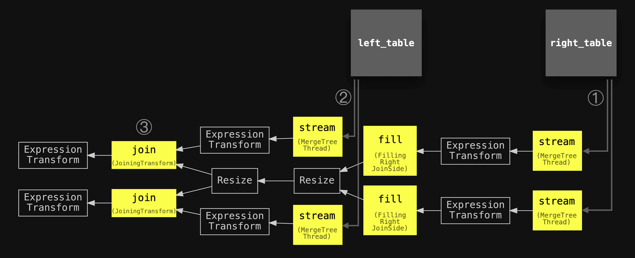
We can see that two concurrent fill stages exist for filling two hash tables with data from the right-hand side table in parallel. Furthermore, two concurrent join stages are used for joining (in the form of hash table lookups) the data from the left-hand side table.
Note that resize stages are used in the query pipeline above for defining explicit connections between all fill and all join stages: All join stages should wait until all fill stages are finished.
Next, we introspect the query pipeline for the parallel hash join query with max_threads set to 4:
./clickhouse client --host ekyyw56ard.us-west-2.aws.clickhouse.cloud --secure --port 9440 --password  --database=imdb_large --query "
EXPLAIN pipeline graph=1, compact=0
SELECT *
FROM actors a
JOIN roles r ON a.id = r.actor_id
SETTINGS max_threads = 4, join_algorithm = 'parallel_hash';" | dot -Tpdf > pipeline.pdf
Now four concurrent fill stages are used for filling four hash tables with data from the right-hand side table in parallel. And four concurrent join stages are used for joining the data from the left-hand side table.
Measurements in the original PR indicate that the speedup is almost linearly correlated to the degree of parallelism.
Grace hash join
Description
Both the hash and parallel hash join algorithms described above are fast but memory-bound. If the right-hand side table doesn’t fit into the main memory, ClickHouse will raise an OOM exception. In this situation, ClickHouse users can sacrifice performance and use a (partial) merge algorithm (described in the next post) that (partially) sorts the table's data into external storage before merging it.
Luckily, ClickHouse 22.12 introduced another join algorithm called ‘grace hash’ that is non-memory bound, but hash table based, and therefore doesn’t require any sorting of the data. This overcomes some of the performance challenges of the (partial) merge algorithm.
The algorithm utilizes a two-phased approach to joining the data. Our implementation differs slightly from the classic algorithmic description in order to fit our query pipeline. The following diagram shows the first phase:
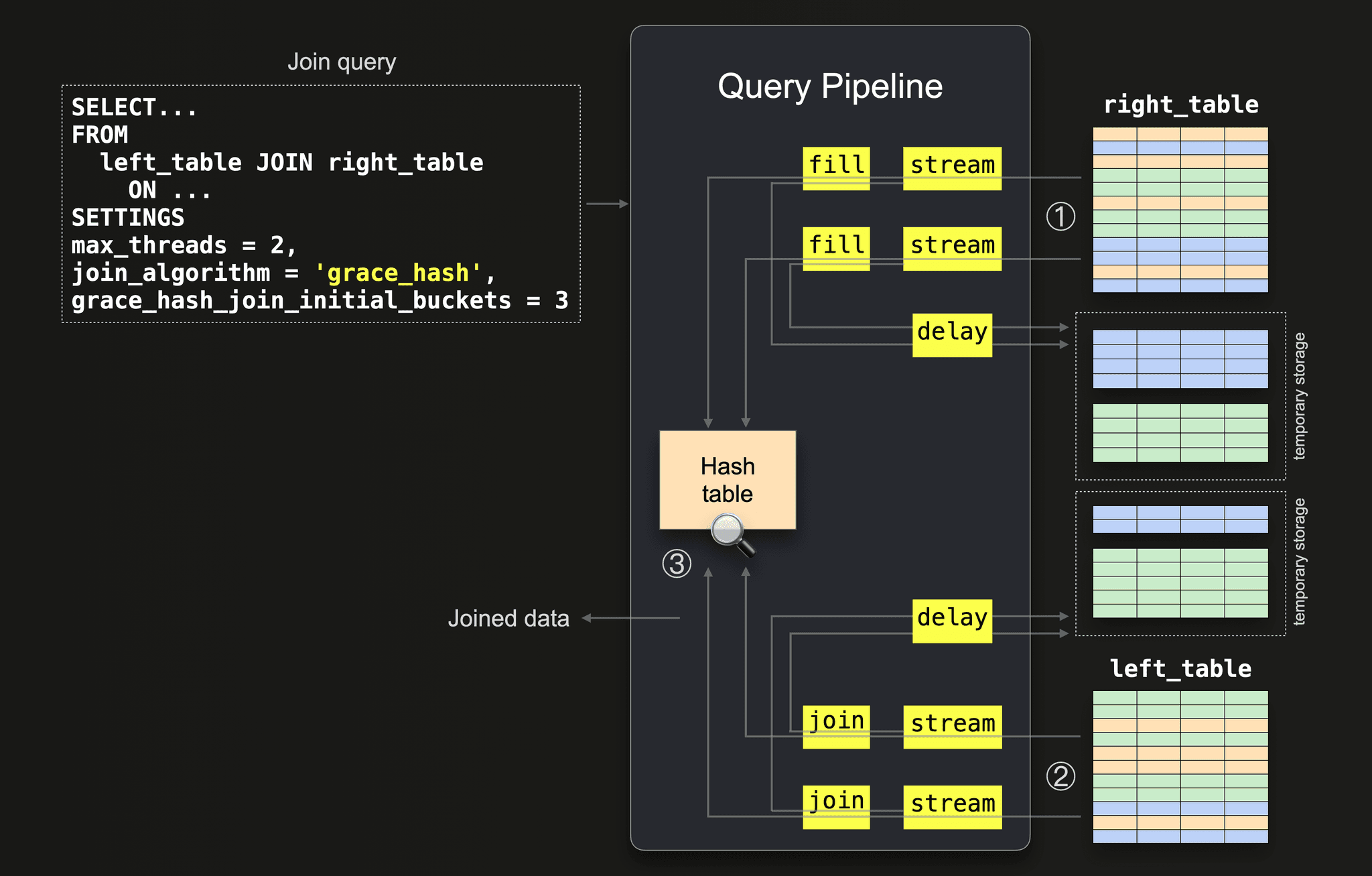
① All data from the right table is streamed block-wise (in parallel by 2 threads because max_threads = 2) into the memory. The rows from each streamed block are split into 3 buckets (because grace_hash_join_initial_buckets = 3) by applying a hash function to the join keys of every row. We sketch this with the orange, blue, and green colors in the diagram above. An in-memory hash table is filled with rows from the first (orange) bucket. The joining of the other two (green and blue) buckets from the right_table is delayed by saving them to temporary storage.
Note that if the in-memory hash table grows beyond the memory limit (as set by max_bytes_in_join), ClickHouse dynamically increases the number of buckets and recomputes the assigned bucket for each row. Any rows which don’t belong to the current bucket are flushed and reassigned.
Also note that ClickHouse rounds the set value for grace_hash_join_initial_buckets up to the closest power of two. Therefore as 3 is rounded up to 4, and 4 initial buckets are used. We use 3 buckets in our diagrams for readability, and there is no crucial difference to the inner workings with 4.
② Data from the left table is streamed in parallel by 2 threads ( max_threads = 2), and the same ‘bucket hash function’ from step ① is applied to the join keys of each row for determining the corresponding bucket. Rows corresponding to the first bucket are ③ joined (as the corresponding hash table is in memory). The joining of the other buckets is delayed by saving them to temporary storage.
The key in steps ① and ② is that the ‘bucket hash function’ will consistently assign values to the same bucket, thereby effectively partitioning the data and solving the problem by decomposition.
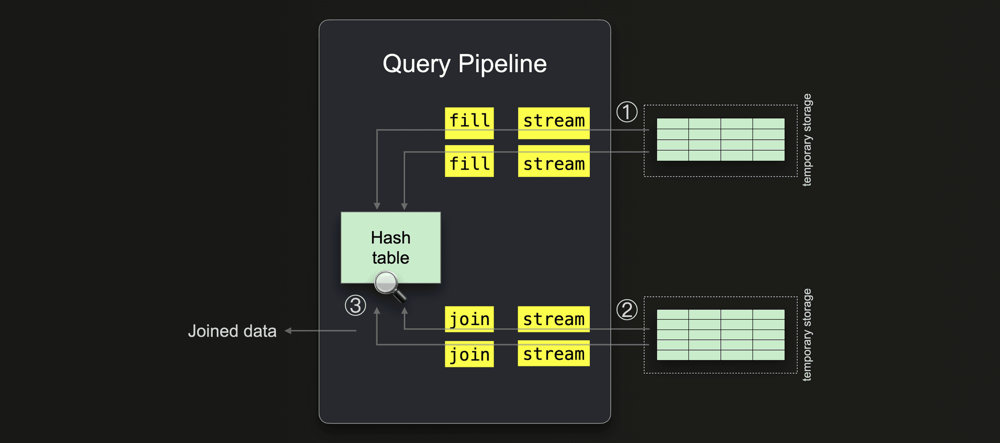
In a second phase, ClickHouse processes the remaining buckets on disk. The remaining buckets are processed sequentially. The following two diagrams sketch this. The first diagram shows how the blue bucket gets processed first. The second diagram shows the processing of the final green bucket.
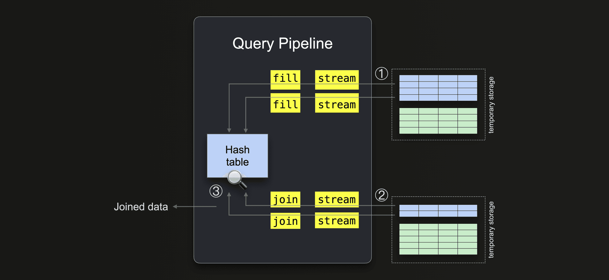
① ClickHouse builds the hash table for each bucket from the right-hand side table data.
Again, if ClickHouse runs out of memory, it dynamically increases the number of buckets.
② Once a hash table has been built from a right-hand side table bucket, ClickHouse streams the data from the corresponding left-hand side table bucket and ③ completes the join for this pair.
Note that during this phase, there can be some rows that belong to another bucket other than the current one, due to them being saved to temporary storage before the number of buckets was dynamically increased. In this case, ClickHouse saves them to the new actual buckets and processes them further.
This process is repeated for all of the remaining buckets.
Supported join types
INNER and LEFT join types and all strictness settings except ASOF are supported.
Examples
Below we compare the runtimes and peak memory consumptions of the same join query run using the hash join and grace hash join algorithms.
Hash join with larger table on the right-hand side:
SELECT *
FROM actors AS a
JOIN roles AS r ON a.id = r.actor_id
FORMAT `Null`
SETTINGS join_algorithm = 'hash';

0 rows in set. Elapsed: 5.038 sec. Processed 101.00 million rows, 3.67 GB (20.05 million rows/s., 727.61 MB/s.)
Grace hash join with larger table on the right-hand side:
SELECT *
FROM actors AS a
JOIN roles AS r ON a.id = r.actor_id
FORMAT `Null`
SETTINGS join_algorithm = 'grace_hash', grace_hash_join_initial_buckets = 3;

0 rows in set. Elapsed: 13.117 sec. Processed 101.00 million rows, 3.67 GB (7.70 million rows/s., 279.48 MB/s.)
We get runtime statistics for the last two query runs:
As expected, the hash join was faster. However, the grace hash join consumed only half of the peak main memory.SELECT query, formatReadableTimeDelta(query_duration_ms / 1000) AS query_duration, formatReadableSize(memory_usage) AS memory_usage, formatReadableQuantity(read_rows) AS read_rows, formatReadableSize(read_bytes) AS read_data FROM clusterAllReplicas(default, system.query_log) WHERE (type = 'QueryFinish') AND hasAll(tables, ['imdb_large.actors', 'imdb_large.roles']) ORDER BY initial_query_start_time DESC LIMIT 2 FORMAT Vertical; Row 1: ────── query: SELECT * FROM actors AS a JOIN roles AS r ON a.id = r.actor_id FORMAT `Null` SETTINGS join_algorithm = 'grace_hash', grace_hash_join_initial_buckets = 3 query_duration: 13 seconds memory_usage: 3.72 GiB read_rows: 101.00 million read_data: 3.41 GiB Row 2: ────── query: SELECT * FROM actors AS a JOIN roles AS r ON a.id = r.actor_id FORMAT `Null` SETTINGS join_algorithm = 'hash' query_duration: 5 seconds memory_usage: 8.96 GiB read_rows: 101.00 million read_data: 3.41 GiB
The main memory consumption of the grace hash join can be reduced further by increasing the grace_hash_join_initial_buckets setting. We demonstrate this by re-running the query with a value of 8 for the grace_hash_join_initial_buckets setting:
SELECT *
FROM actors AS a
JOIN roles AS r ON a.id = r.actor_id
FORMAT `Null`
SETTINGS join_algorithm = 'grace_hash', grace_hash_join_initial_buckets = 8;

0 rows in set. Elapsed: 16.366 sec. Processed 101.00 million rows, 3.67 GB (6.17 million rows/s., 224.00 MB/s.)
Let’s check runtime statistics for the last two query runs:
SELECT
    query,
    formatReadableTimeDelta(query_duration_ms / 1000) AS query_duration,
    formatReadableSize(memory_usage) AS memory_usage,
    formatReadableQuantity(read_rows) AS read_rows,
    formatReadableSize(read_bytes) AS read_data
FROM clusterAllReplicas(default, system.query_log)
WHERE (type = 'QueryFinish') AND hasAll(tables, ['imdb_large.actors', 'imdb_large.roles'])
ORDER BY initial_query_start_time DESC
LIMIT 2
FORMAT Vertical;

Row 1:
──────
query:          SELECT *
                FROM actors AS a
                JOIN roles AS r ON a.id = r.actor_id
                FORMAT `Null`
                SETTINGS join_algorithm = 'grace_hash', grace_hash_join_initial_buckets = 8
query_duration: 16 seconds
memory_usage:   2.10 GiB
read_rows:      101.00 million
read_data:      3.41 GiB

Row 2:
──────
query:          SELECT *
                FROM actors AS a
                JOIN roles AS r ON a.id = r.actor_id
                FORMAT `Null`
                SETTINGS join_algorithm = 'grace_hash', grace_hash_join_initial_buckets = 3
query_duration: 13 seconds
memory_usage:   3.72 GiB
read_rows:      101.00 million
read_data:      3.41 GiB
The run of grace hash join with 8 initial buckets consumed roughly 70% less main memory than the run with 3 initial buckets. For the sacrifice of higher execution time, the memory consumption can be reduced quite linearly by increasing the number of buckets.
Note that, as mentioned before and demonstrated below, ClickHouse always rounds the set value for grace_hash_join_initial_buckets up to the closest power of two. Therefore the query run with grace_hash_join_initial_buckets set to 3 is actually using 4 initial buckets.
Query pipeline
We introspect the query pipeline for a grace hash join query with max_threads set to 2 and grace_hash_join_initial_buckets set to 3:
./clickhouse client --host ekyyw56ard.us-west-2.aws.clickhouse.cloud --secure --port 9440 --password  --database=imdb_large --query "
EXPLAIN pipeline graph=1, compact=0
SELECT *
FROM actors AS a
JOIN roles AS r ON a.id = r.actor_id
FORMAT `Null`
SETTINGS max_threads = 2, join_algorithm = 'grace_hash', grace_hash_join_initial_buckets = 3';" | dot -Tpdf > pipeline.pdf
The added circled numbers and slightly simplified names of the main stages and added two joined tables are used for aligning with the abstract diagram above:
We see that ① with two parallel stream stages (max_threads=2), data from the right-hand side table is streamed into the memory. We also see two parallel fill stages being used for filling an in-memory hash table. Two additional parallel stream stages ② and two parallel join stages ③ are used for streaming and joining data from the left-hand side table. A delay stage indicates that some of the joining stages are postponed.
However, we can’t see the number of buckets in the query pipeline since the creation of buckets is dynamic and depends on memory pressure with ClickHouse dynamically increasing the number as required. All of the buckets are processed in the Delayed…Transform stages.
In order to introspect the number of created and processed buckets, we need to introspect the actual execution of the grace hash join query, by asking ClickHouse to send trace-level logs during the execution to the ClickHouse command line client.
We execute the grace hash join query with a max_threads setting of 2 and a grace_hash_join_initial_buckets value of 3 (note the send_logs_level='trace' setting):
./clickhouse client --host ea3kq2u4fm.eu-west-1.aws.clickhouse.cloud --secure --password  --database=imdb_large --send_logs_level='trace' --query "
SELECT *
FROM actors AS a
JOIN roles AS r ON a.id = r.actor_id
FORMAT Null
SETTINGS max_threads = 2, join_algorithm = 'grace_hash', grace_hash_join_initial_buckets = 3;"

    ...
... GraceHashJoin: Initialize 4 buckets
... GraceHashJoin: Joining file bucket 0
    ...
... imdb_large.actors ...: Reading approx. 1000000 rows with 2 streams
    ...
... imdb_large.roles ...: Reading approx. 100000000 rows with 2 streams
    ...
... GraceHashJoin: Joining file bucket 1
... GraceHashJoin: Loaded bucket 1 with 250000(/25000823) rows
    ...
... GraceHashJoin: Joining file bucket 2
... GraceHashJoin: Loaded bucket 2 with 250000(/24996460) rows
    ...
... GraceHashJoin: Joining file bucket 3
... GraceHashJoin: Loaded bucket 3 with 250000(/25000742) rows
    ...
... GraceHashJoin: Finished loading all 4 buckets
    ...
We can now see that 4 (instead of 3) initial buckets were created. Because, as mentioned before, ClickHouse always rounds the set value for grace_hash_join_initial_buckets up to the closest power of two. We also see how 2 parallel stream stages are used per table for reading the table’s rows. The first corresponding bucket (bucket 0 in the trace log messages above) of both tables gets immediately joined.
The other 3 buckets are written to disk, and later sequentially loaded for joining. We see that the 1 million, and the 100 million rows from both tables were evenly split - 250 thousand rows, and ~25 million rows, respectively, per bucket.
For comparison, we execute the grace hash join query with a max_threads setting of 4 and a grace_hash_join_initial_buckets value of 8:
./clickhouse client --host ea3kq2u4fm.eu-west-1.aws.clickhouse.cloud --secure --password  --database=imdb_large --send_logs_level='trace' --query "
SELECT *
FROM actors AS a
JOIN roles AS r ON a.id = r.actor_id
FORMAT Null
SETTINGS max_threads = 4, join_algorithm = 'grace_hash', grace_hash_join_initial_buckets = 8;"

    ...
... GraceHashJoin: Initialize 8 buckets
... GraceHashJoin: Joining file bucket 0
    ...
... imdb_large.actors ...: Reading approx. 1000000 rows with 4 streams
    ...
... imdb_large.roles ...: Reading approx. 100000000 rows with 4 streams
    ...
...  GraceHashJoin: Joining file bucket 1
...  GraceHashJoin: Loaded bucket 1 with 125000(/12502068) rows
    ...
...  GraceHashJoin: Joining file bucket 2
...  GraceHashJoin: Loaded bucket 2 with 125000(/12498406) rows
    ...
...  GraceHashJoin: Joining file bucket 3
...  GraceHashJoin: Loaded bucket 3 with 125000(/12502699) rows
    ...
...  GraceHashJoin: Joining file bucket 4
...  GraceHashJoin: Loaded bucket 4 with 125000(/12498074) rows
    ...
...  GraceHashJoin: Joining file bucket 5
...  GraceHashJoin: Loaded bucket 5 with 125000(/12498755) rows
    ...
...  GraceHashJoin: Joining file bucket 6
...  GraceHashJoin: Loaded bucket 6 with 125000(/12498054) rows
    ...
...  GraceHashJoin: Joining file bucket 7
...  GraceHashJoin: Loaded bucket 7 with 125000(/12498043) rows
    ...
...  GraceHashJoin: Finished loading all 8 buckets
    ...
We can see that 8 initial buckets were created and that 4 parallel stream stages were used per table for reading the table’s rows.
Summary
This blog post described and compared in detail the 3 ClickHouse join algorithms that are based on in-memory hash tables.
The Hash join algorithm is fast and the most generic one supporting all join types and strictness settings, but the creation of the in-memory hash table is single-threaded, and can become a bottleneck if the right-hand side table is very large.
The Parallel hash join algorithm can be faster with large right-hand side tables by building several hash tables concurrently, but requires more memory.
The Grace hash join algorithm is a non-memory bound version, that splits the input data into buckets, with some of them being offloaded to disk before being processed in-memory sequentially.
The following chart summarizes the memory consumption and execution times of all join query runs (with max_threads set to 30 and the larger table on the right-hand side) from this post:
In the next parts of this series, we will explore the remaining 3 join algorithms available in ClickHouse:
- Full sorting merge join
- Partial merge join
- Direct join
Stay tuned!
Get started with ClickHouse Cloud today and receive $300 in credits. At the end of your 30-day trial, continue with a pay-as-you-go plan, or contact us to learn more about our volume-based discounts. Visit our pricing page for details.


