You can find updated guidance on ClickHouse query optimization for 2026 and beyond in The definitive guide to ClickHouse query optimization
Introduction #
ClickHouse is a blazingly fast relational database management system optimized for real-time analytics. Even though queries are typically fast enough with little to no tuning, we believe in the principle that no miliseconds should be waisted! In this post we'll give you some tips on how to accelerate your ClickHouse queries and make them even faster than ever, using some practical examples.
A quick ClickHouse query processing primer #
Tables in ClickHouse are designed to receive millions of row inserts per second and to store very large (100s of Petabytes) volumes of data.
Fast query speed in ClickHouse is usually achieved by properly utilizing a table’s (sparse) primary index in order to drastically limit the amount of data ClickHouse needs to read from disk and in order to prevent resorting of data at query time which also can enable short-circuiting when a LIMIT clause is used.
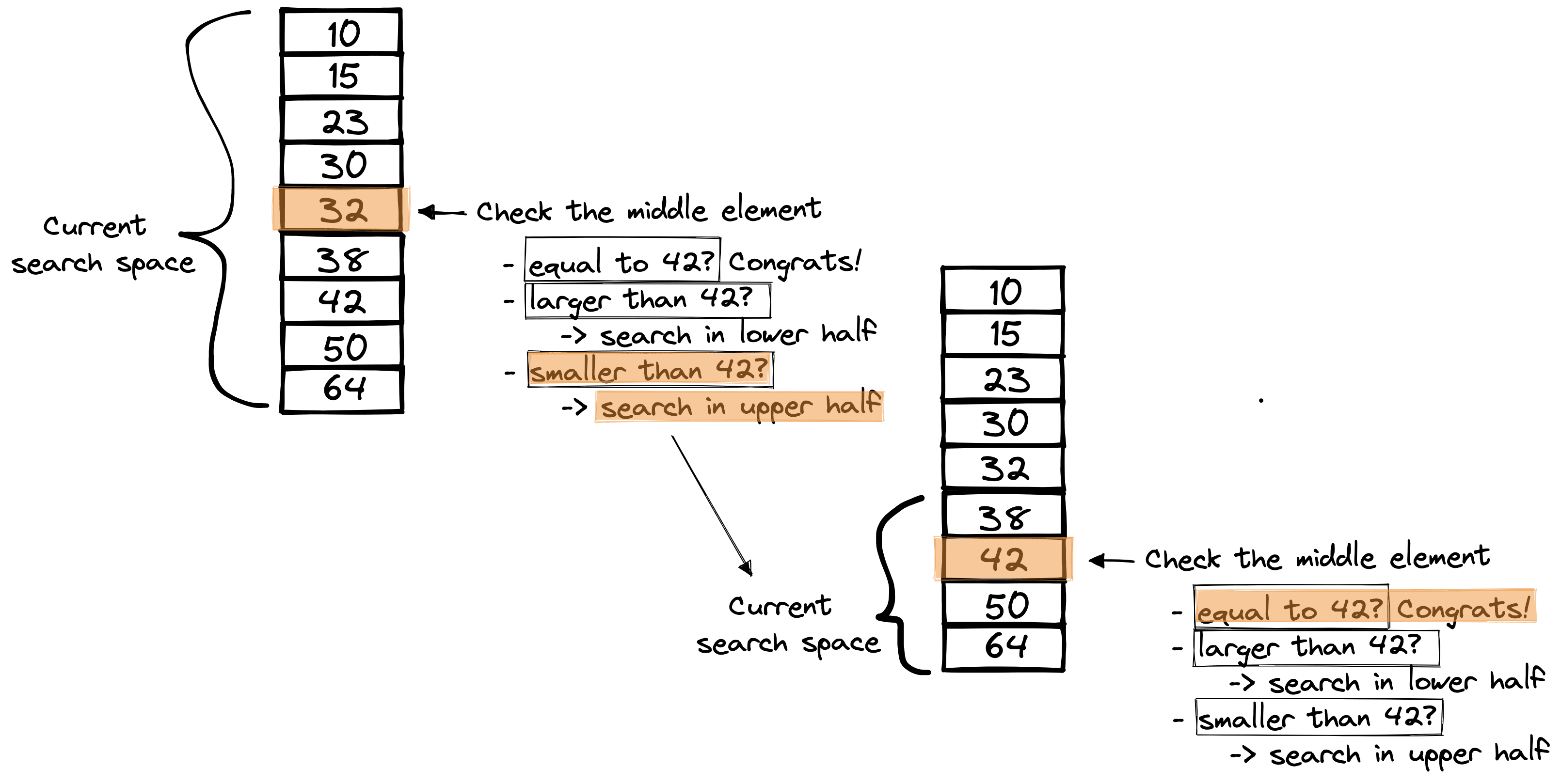
The design of the ClickHouse primary index is based on the binary search algorithm, that efficiently (time complexity of O(log2 n)) finds the position of a target value within a sorted array.
For example, consider the sorted array in the diagram below, where the binary search algorithm is used to find the value 42. The algorithm compares the target value 42 to the middle element of the array. If they are not equal, the half in which the target cannot lie is eliminated, and the search continues on the remaining half, again taking the middle element to compare to the target value, and repeating this until the target value is found:
Finding rows in a ClickHouse table with the table’s primary index works in the same way.
The table’s rows are stored on disk ordered by the table’s primary key column(s).
Based on that row order, the primary index (which is a sorted array like in the diagram above) stores the primary key column value(s) from each 8192nd row of the table.
In the diagram below, we assume a table with a column ‘numbers’, which is also the primary key column:
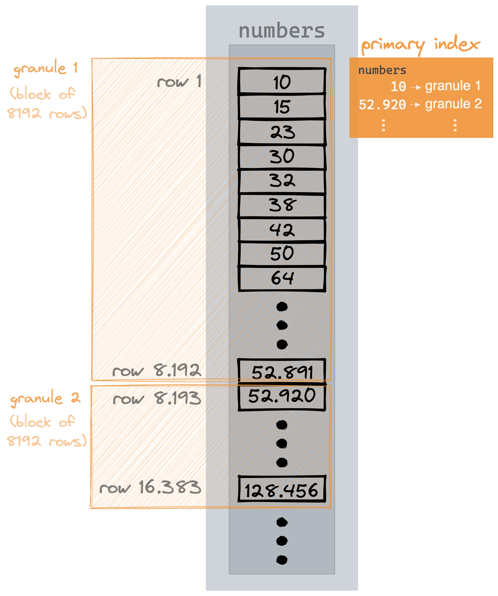
Instead of indexing individual rows, the ClickHouse primary index is indexing blocks of rows (so-called granules).
With such a primary index, terabytes or even petabytes of data can be skipped and thus searched in a matter of (sub-) seconds.
The following diagram shows how ClickHouse typically executes a query:
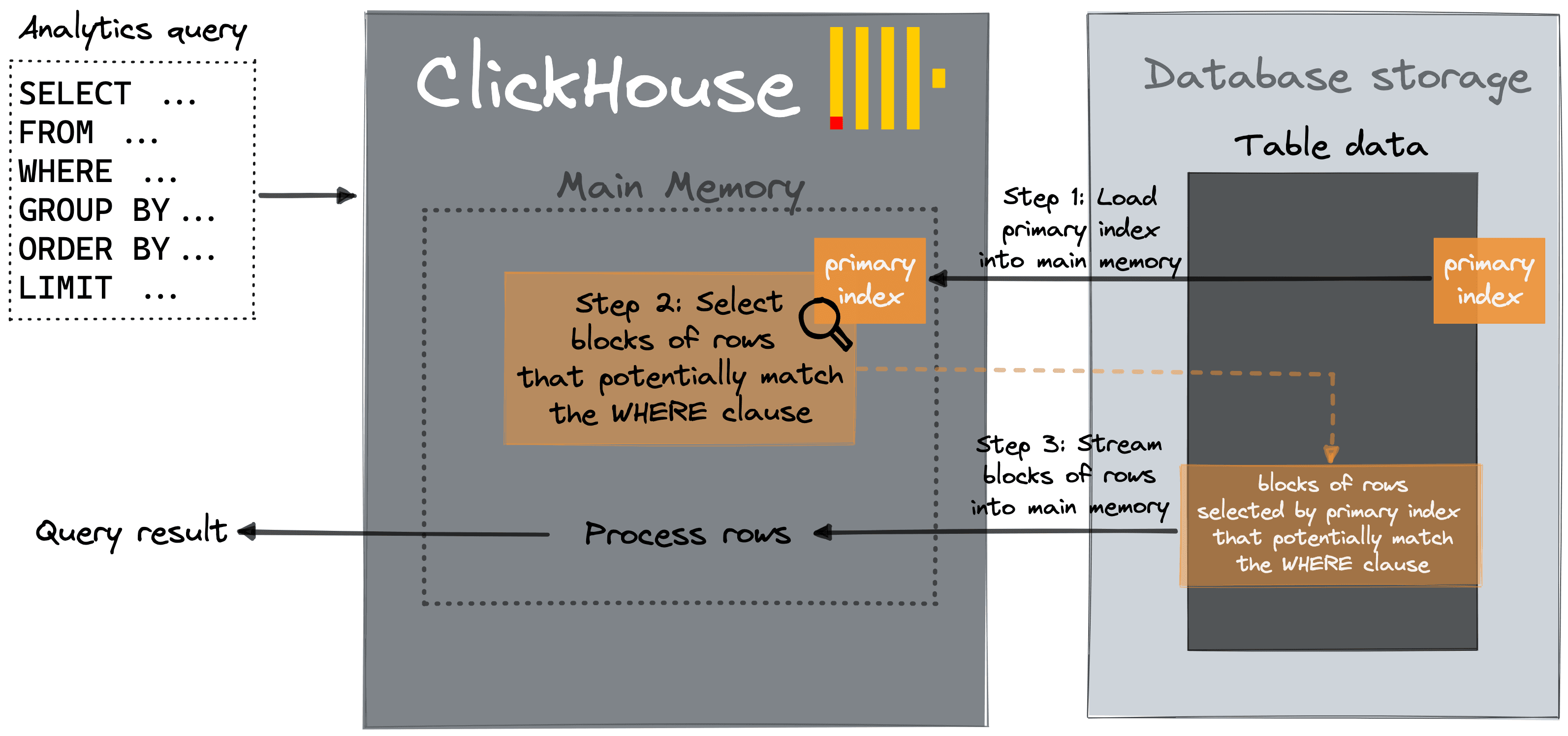
Step 1: The primary index from the involved table is loaded into the main memory.
Step 2: Typically, via a binary search over the index entries, ClickHouse selects blocks of rows that potentially contain rows matching the query’s WHERE clause.
Step 3: The selected blocks of rows are streamed in parallel into the ClickHouse query engine for further processing, and the query result is streamed to the caller.
There are three main tuning knobs for speeding up this query execution workflow in ClickHouse:
The less data ClickHouse needs to stream from disk to main memory, the faster the query’s execution time will be. The amount of data required to be streamed from disk can be minimized by (1) properly utilizing primary indexes and (2) pre-computing aggregates.
The streaming and actual processing of the data can be sped up by (3) increasing the level of parallelism used inside the ClickHouse query processing engine.
(1) Properly utilize primary indexes #
Lets first look at how we can ensure primary indexes are fully utilized to ensure optimal query performance.
Utilize indexes for minimizing the amount of data to be streamed into ClickHouse #
As a running example, we use the table from our UK Property Price Paid tutorial with 27.64 million rows. This dataset is available within our sql.clickhouse.com environment.
We run a query that lists the counties in London for the three highest paid prices:
SELECT county, price FROM uk_price_paid WHERE town = 'LONDON' ORDER BY price DESC LIMIT 3 ┌─county─────────┬─────price─┐ │ GREATER LONDON │ 594300000 │ │ GREATER LONDON │ 569200000 │ │ GREATER LONDON │ 448500000 │ └────────────────┴───────────┘ 3 rows in set. Elapsed: 0.044 sec. Processed 27.64 million rows, 44.21 MB (634.60 million rows/s., 1.01 GB/s.)✎
ClickHouse is doing a full table scan!
Because the primary index of the table can’t be properly utilized for the query.
We check the primary key of the table:
SHOW CREATE TABLE uk_price_paid CREATE TABLE default.uk_price_paid ( `price` UInt32, `date` Date, `postcode1` LowCardinality(String), `postcode2` LowCardinality(String), `type` Enum8('other' = 0, 'terraced' = 1, 'semi-detached' = 2, 'detached' = 3, 'flat' = 4), `is_new` UInt8, `duration` Enum8('unknown' = 0, 'freehold' = 1, 'leasehold' = 2), `addr1` String, `addr2` String, `street` LowCardinality(String), `locality` LowCardinality(String), `town` LowCardinality(String), `district` LowCardinality(String), `county` LowCardinality(String), `category` UInt8 ) ENGINE = ReplicatedMergeTree('/clickhouse/tables/fb100991-4cae-4a92-995a-1ca11416879e/{shard}', '{replica}') ORDER BY (postcode1, postcode2, addr1, addr2) SETTINGS index_granularity = 8192 1 row in set. Elapsed: 0.001 sec.✎
The tables ORDER BY clause determines how the data is ordered on disk, and the primary index entries. The columns in the ORDER BY are postcode1, postcode2, addr1, and addr2.
Note that ClickHouse uses the sorting key (defined by the ORDER BY clause) as the primary key if the latter is not defined explictly i.e. via a PRIMARY KEY clause.
That doesn’t help for the query with the town = 'LONDON' predicate.
If we want to significantly speed up our sample query that filters for rows with a specific town, then we need to use a primary index optimized for that query.
One option is to create a second table with a different row order based on a different primary key.
Because a table can only have one physical order on disk, we need to duplicate the table data into another table.
We create a second table with the same schema as the original table but with a different primary key, and we copy the data between the tables:
CREATE TABLE uk_price_paid_oby_town_price
(
    price UInt32,
    date Date,
    postcode1 LowCardinality(String),
    postcode2 LowCardinality(String),
    type Enum8('terraced' = 1, 'semi-detached' = 2, 'detached' = 3, 'flat' = 4, 'other' = 0),
    is_new UInt8,
    duration Enum8('freehold' = 1, 'leasehold' = 2, 'unknown' = 0),
    addr1 String,
    addr2 String,
    street LowCardinality(String),
    locality LowCardinality(String),
    town LowCardinality(String),
    district LowCardinality(String),
    county LowCardinality(String),
    category UInt8
)
ENGINE = MergeTree
ORDER BY (town, price);

INSERT INTO uk_price_paid_oby_town_price
SELECT * FROM uk_price_paid;

0 rows in set. Elapsed: 13.033 sec. Processed 52.50 million rows, 2.42 GB (4.03 million rows/s., 185.58 MB/s.)
We run the query on the second table:
SELECT county, price FROM uk_price_paid_oby_town_price WHERE town = 'LONDON' ORDER BY price DESC LIMIT 3 ┌─county─────────┬─────price─┐ │ GREATER LONDON │ 594300000 │ │ GREATER LONDON │ 569200000 │ │ GREATER LONDON │ 448500000 │ └────────────────┴───────────┘ 3 rows in set. Elapsed: 0.005 sec. Processed 81.92 thousand rows, 493.76 KB (15.08 million rows/s., 90.87 MB/s.)✎
Much better.
Utilize indexes for preventing resorting and enabling short-circuiting #
In our previous example, ClickHouse is not only streaming much less data from disk but is applying an additional optimization.
The query is:
- Filtering rows for town = ‘London’
- Ordering the matching rows by price descending
- Getting the top 3 rows
For this, normally, ClickHouse:
- uses the primary index for selecting blocks that potentially contain ‘London’ rows and streams these rows from disk
- orders these rows in main memory by price
- streams the top 3 rows as the result to the caller
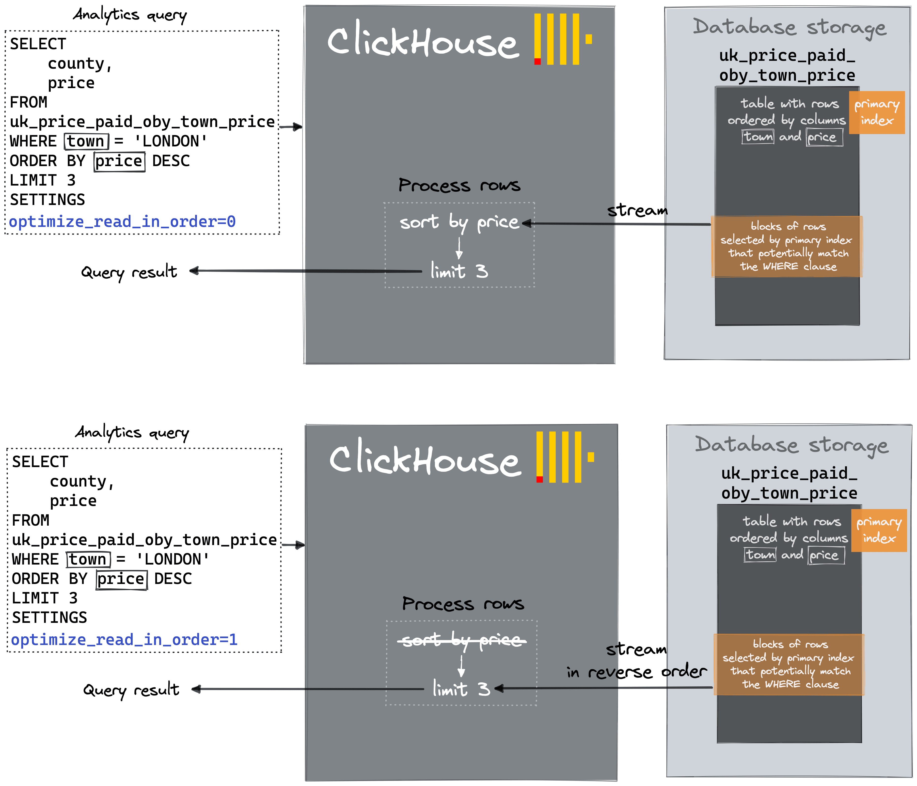
But, because the ‘London’ rows on disk are stored already ordered by price (see the table DDL’s ORDER BY clause), ClickHouse can just skip the resorting in main memory.
And ClickHouse can do short-circuiting. All ClickHouse has to do, is to stream the selected blocks of rows from disk in reverse order, and once three matching (town = ‘London’) rows have been streamed, the query is done.
This is exactly what the optimize_read_in_order optimization is doing in this case - preventing resorting of the rows and enabling short-circuiting.
This optimization is enabled by default, and when we inspect the logical query plan of the query via EXPLAIN, we can see ReadType: InReverseOrder at the bottom of the plan:
EXPLAIN actions = 1 SELECT county, price FROM uk_price_paid_oby_town_price WHERE town = 'LONDON' ORDER BY price DESC LIMIT 3 Expression (Projection) Actions: INPUT :: 0 -> price UInt32 : 0 INPUT :: 1 -> county LowCardinality(String) : 1 Positions: 1 0 Limit (preliminary LIMIT (without OFFSET)) Limit 3 Offset 0 Sorting (Sorting for ORDER BY) Prefix sort description: price DESC Result sort description: price DESC Limit 3 Expression (Before ORDER BY) Actions: INPUT :: 0 -> price UInt32 : 0 INPUT :: 1 -> county LowCardinality(String) : 1 Positions: 0 1 Filter (WHERE) Filter column: equals(town, 'LONDON') (removed) Actions: INPUT :: 0 -> price UInt32 : 0 INPUT : 1 -> town LowCardinality(String) : 1 INPUT :: 2 -> county LowCardinality(String) : 2 COLUMN Const(String) -> 'LONDON' String : 3 FUNCTION equals(town :: 1, 'LONDON' :: 3) -> equals(town, 'LONDON') LowCardinality(UInt8) : 4 Positions: 0 2 4 ReadFromMergeTree (default.uk_price_paid_oby_town_price) ReadType: InReverseOrder Parts: 6 Granules: 267 27 rows in set. Elapsed: 0.002 sec.✎
The optimize_read_in_order setting can be disabled via the SETTINGS clause of the query. This will cause ClickHouse to stream 2.17 million rows instead of 81.92 thousand rows from disk (still better than a full table scan). The following diagram visualizes the difference in query processing steps:
One remaining issue with using a second table with a different row order is keeping the tables in sync. Further below, we will discuss a handy solution for this problem.
(2) Pre-compute aggregates #
We execute an aggregation query that lists the U.K. counties with the three highest average paid prices:
SELECT county, avg(price) FROM uk_price_paid GROUP BY county ORDER BY avg(price) DESC LIMIT 3 ┌─county──────────────────────────────┬─────────avg(price)─┐ │ WINDSOR AND MAIDENHEAD │ 383843.17329304793 │ │ BOURNEMOUTH, CHRISTCHURCH AND POOLE │ 383478.9135281004 │ │ GREATER LONDON │ 376911.4824869095 │ └─────────────────────────────────────┴────────────────────┘ 3 rows in set. Elapsed: 0.020 sec. Processed 26.25 million rows, 132.57 MB (1.33 billion rows/s., 6.69 GB/s.)✎
In this case, ClickHouse is doing a full table scan because the query aggregates all existing table rows. Therefore the primary index can’t be used to reduce the amount of data streamed from disk.
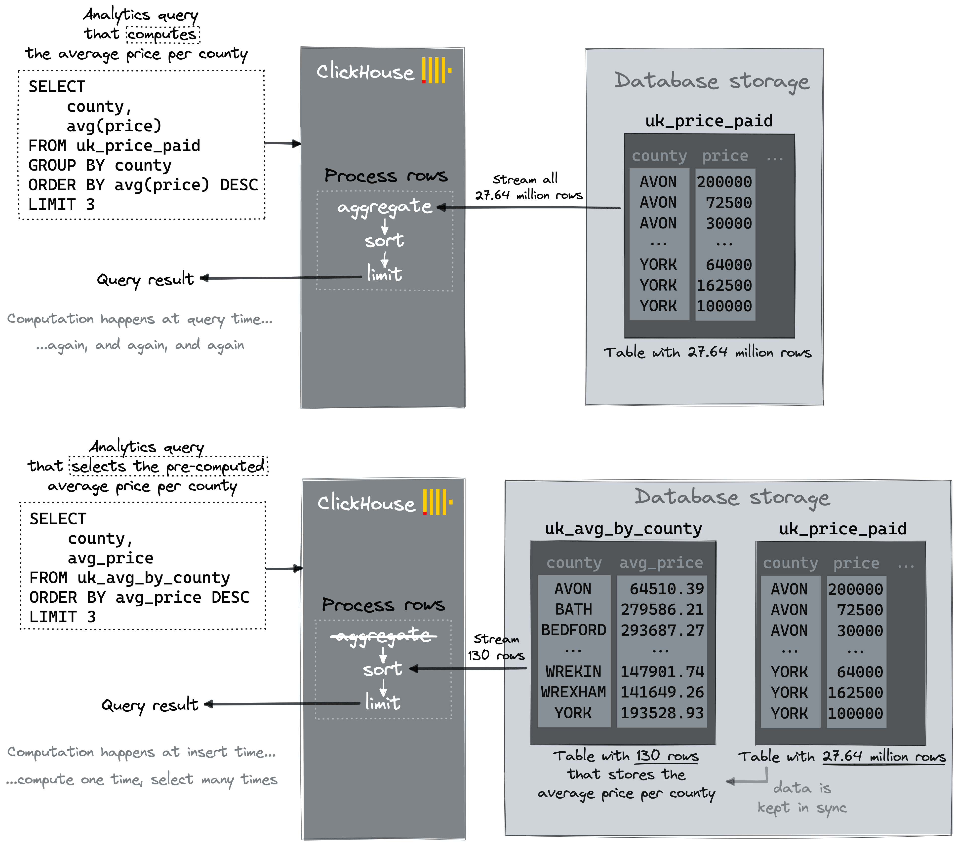
However, we could drastically reduce the amount of data streamed from disk (by sacrificing additional disk space) if we could pre-compute the aggregate values for all existing 130 U.K counties in a separate table and update that separate table, whenever the original table data changes.
The following diagram visualizes this idea:
ClickHouse has a handy new turnkey feature implementing this idea: Projections!
Use projections for (1) and (2) #
A ClickHouse table can have (multiple) projections.
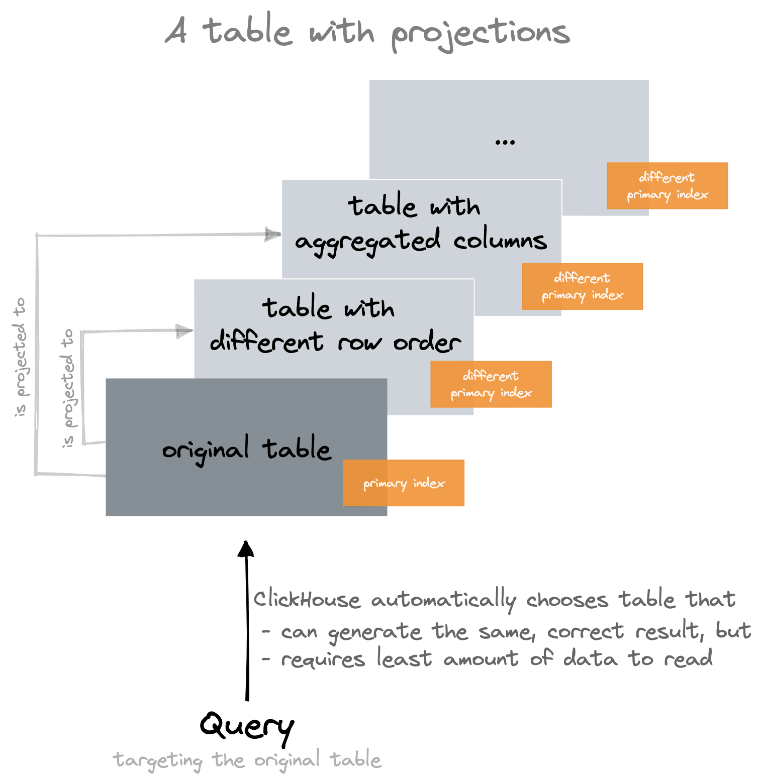
A projection is an additional (hidden) table that is automatically kept in sync with the original table. The projection can have a different row order (and therefore a different primary index) than the original table, as well as automatically and incrementally pre-compute aggregate values.
When a query is targeting the original table, then ClickHouse automatically chooses (by sampling the primary keys) a table that can generate the same correct result, but requires the least amount of data to be read. We visualize this concept here:
Projections are somewhat similar to Materialized Views, which also allow you to have incremental aggregation and multiple row orders. But unlike Materialized Views, projections are updated atomically and kept consistent with the main table with ClickHouse automatically choosing the optimal version at query time.
For the original example table uk_price_paid, we will create (and populate) two projections.
In order to keep things tidy and simple in our playground, we first duplicate the table uk_price_paid as uk_price_paid_with_projections:
CREATE TABLE uk_price_paid_with_projections AS uk_price_paid;
INSERT INTO uk_price_paid_with_projections SELECT * FROM uk_price_paid;

0 rows in set. Elapsed: 4.410 sec. Processed 52.50 million rows, 2.42 GB (11.90 million rows/s., 548.46 MB/s.)
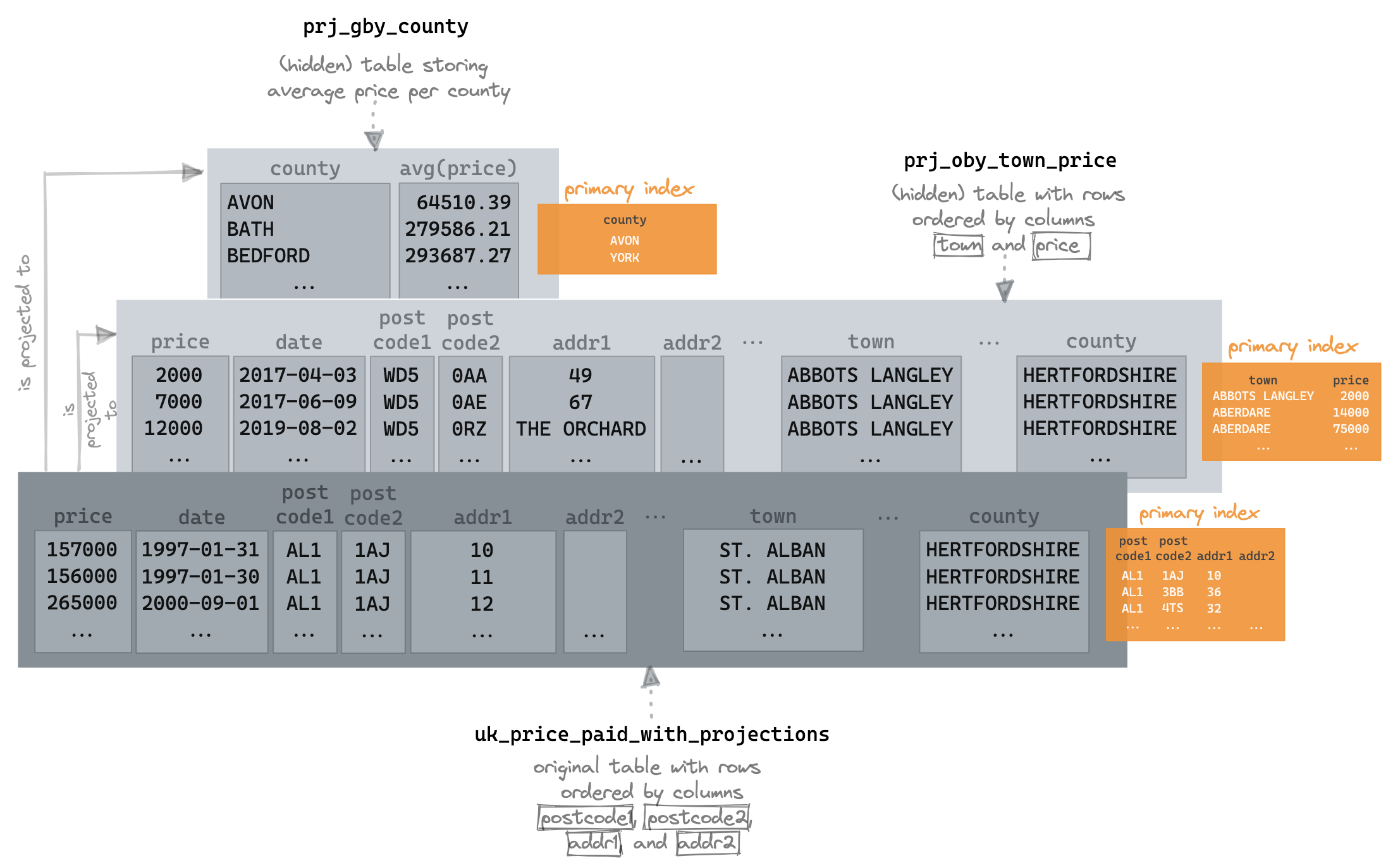
We create and populate projection prj_oby_town_price – an additional (hidden) table with a primary index, ordering by town and price, to optimize the query that lists the counties in a specific town for the highest paid prices:
ALTER TABLE uk_price_paid_with_projections
    ADD PROJECTION prj_oby_town_price
    (
        SELECT
            *
        ORDER BY
          town, price
    );

ALTER TABLE uk_price_paid_with_projections
    MATERIALIZE PROJECTION prj_oby_town_price SETTINGS mutations_sync = 1;

0 rows in set. Elapsed: 6.028 sec.
We create and populate projection prj_gby_county – an additional (hidden) table that incrementally pre-computes the avg(price) aggregate values for all existing 130 U.K counties:
ALTER TABLE uk_price_paid_with_projections
    ADD PROJECTION prj_gby_county
    (
        SELECT
            county,
            avg(price)
        GROUP BY
           county
    );

ALTER TABLE uk_price_paid_with_projections
    MATERIALIZE PROJECTION prj_gby_county SETTINGS mutations_sync = 1;

0 rows in set. Elapsed: 0.123 sec.
Note that If there is a GROUP BY clause used in a projection (like in the prj_gby_county above), the underlying storage engine for the (hidden) table becomes AggregatingMergeTree, and all aggregate functions are converted to AggregateFunction. This ensures proper incremental data aggregation.
Also, note the SETTINGS clause that forces synchronous execution.
This is a visualization of the main table uk_price_paid_with_projections and its two projections:
If we now run the query that lists the counties in London for the three highest paid prices, we see a dramatic difference in performance:
SELECT county, price FROM uk_price_paid_with_projections WHERE town = 'LONDON' ORDER BY price DESC LIMIT 3 ┌─county─────────┬─────price─┐ │ GREATER LONDON │ 594300000 │ │ GREATER LONDON │ 569200000 │ │ GREATER LONDON │ 448500000 │ └────────────────┴───────────┘ 3 rows in set. Elapsed: 0.026 sec. Processed 2.17 million rows, 13.03 MB (83.14 million rows/s., 499.14 MB/s.)✎
Likewise, for the query that lists the U.K. counties with the three highest average paid prices:
SELECT county, avg(price) FROM uk_price_paid_with_projections GROUP BY county ORDER BY avg(price) DESC LIMIT 3 ┌─county──────────────────────────────┬─────────avg(price)─┐ │ WINDSOR AND MAIDENHEAD │ 398334.9180566017 │ │ GREATER LONDON │ 396401.2740568222 │ │ BOURNEMOUTH, CHRISTCHURCH AND POOLE │ 387441.28323942184 │ └─────────────────────────────────────┴────────────────────┘ 3 rows in set. Elapsed: 0.007 sec.✎
Note that both queries target the original table, and that both queries resulted in a full table scan (all 27.64 million rows got streamed from disk) before we created the two projections.
Also, note that the query that lists the counties in London for the three highest paid prices is streaming 2.17 million rows. When we directly used a second table optimized for this query, only 81.92 thousand rows were streamed from disk.
The reason for the difference is that currently, the optimize_read_in_order optimization mentioned above isn’t supported for projections.
We inspect the system.query_log table in order to see that ClickHouse automatically used the two projections for the two queries above (see the projections column below):
SELECT
    tables,
    query,
    query_duration_ms::String ||  ' ms' AS query_duration,
    formatReadableQuantity(read_rows) AS read_rows,
    projections
FROM clusterAllReplicas(default, system.query_log)
WHERE (type = 'QueryFinish') AND (tables = ['default.uk_price_paid_with_projections'])
ORDER BY initial_query_start_time DESC
LIMIT 2
FORMAT Vertical

Row 1:
──────
tables:         ['default.uk_price_paid_with_projections']
query:          SELECT
                  county,
                  avg(price)
                FROM uk_price_paid
                GROUP BY county
                ORDER BY avg(price) DESC
                LIMIT 3
query_duration: 6 ms
read_rows:      597.00
projections:    ['default.uk_price_paid.prj_gby_county']

Row 2:
──────
tables:         ['default.uk_price_paid_with_projections']
query:          SELECT
                  county,
                  price
                FROM uk_price_paid
                WHERE town = 'LONDON'
                ORDER BY price DESC
                LIMIT 3
query_duration: 25 ms
read_rows:      2.17 million
projections:    ['default.prj_oby_town_price']
Increase query processing parallelism #
Most analytical queries have a filter, aggregation, and sort stage. Each of these can be parallelized independently and will, by default, use as many threads as CPU cores, thus utilizing the full machine resources for a query (Therefore, in ClickHouse, scaling up is preferred to scaling out).
A query sent to ClickHouse gets transformed into a physical query plan, called a query pipeline, which consists of query processing stages that are executed over the data streamed from disk.
As mentioned in the first paragraph, for executing a query, ClickHouse first uses the primary index for selecting blocks of rows that potentially contain rows matching the query’s WHERE clause.
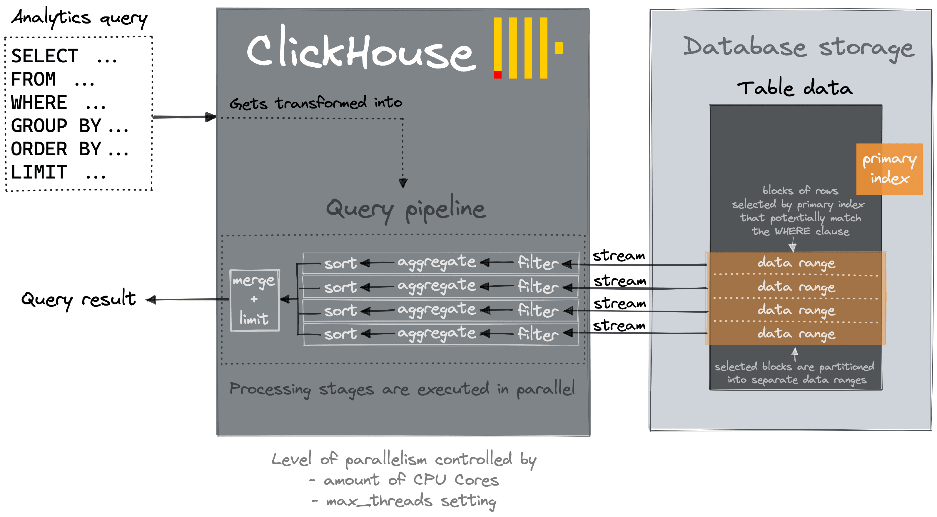
The selected blocks of rows are partitioned into n separate data ranges.
n is dependent on the max_threads setting, which by default is set to the number of CPU cores that ClickHouse sees on the machine it is running on.
In parallel, one thread per data range will read the rows from its range block-wise in a streaming fashion. Most query processing stages from the query pipeline are executed by n threads in parallel in a streaming fashion.
We visualize this for a ClickHouse node with 4 CPU cores:
By increasing the max_threads setting for a query, the level of parallelism for data processing is increased.
We can inspect the query pipeline of a query via EXPLAIN:
EXPLAIN PIPELINE SELECT county, price FROM uk_price_paid WHERE town = 'LONDON' ORDER BY price DESC LIMIT 3 ┌─explain─────────────────────────────────┐ │ (Expression) │ │ ExpressionTransform │ │ (Limit) │ │ Limit │ │ (Sorting) │ │ MergingSortedTransform 4 → 1 │ │ MergeSortingTransform × 4 │ │ LimitsCheckingTransform × 4 │ │ PartialSortingTransform × 4 │ │ (Expression) │ │ ExpressionTransform × 4 │ │ (ReadFromMergeTree) │ │ MergeTreeThread × 4 0 → 1 │ └─────────────────────────────────────────┘ 13 rows in set. Elapsed: 0.002 sec.✎
The plan can be read from bottom to top, and we can see that 4 parallel threads are used for reading/streaming the selected blocks of rows from disk and that most query processing stages from the query pipeline are executed by 4 threads in parallel.
4 threads because the EXPLAIN query was run on a ClickHouse node with 4 CPU cores, and therefore max_threads is set to 4 by default:
SELECT *
FROM system.settings
WHERE name = 'max_threads'
FORMAT Vertical

Row 1:
──────
name:        max_threads
value:       4
changed:     0
description: The maximum number of threads to execute the request. By default, it is determined automatically.
min:         ᴺᵁᴸᴸ
max:         ᴺᵁᴸᴸ
readonly:    0
type:        MaxThreads

1 row in set. Elapsed: 0.009 sec.
We inspect the query pipeline again for the same query that now has a SETTINGS clause increasing the max_threads setting to 20:
EXPLAIN PIPELINE
SELECT
    county,
    price
FROM uk_price_paid
WHERE town = 'LONDON'
ORDER BY price DESC
LIMIT 3
SETTINGS max_threads = 20

┌─explain──────────────────────────────────┐
│ (Expression)                             │
│ ExpressionTransform                      │
│   (Limit)                                │
│   Limit                                  │
│     (Sorting)                            │
│     MergingSortedTransform 20 → 1        │
│       MergeSortingTransform × 20         │
│         LimitsCheckingTransform × 20     │
│           PartialSortingTransform × 20   │
│             (Expression)                 │
│             ExpressionTransform × 20     │
│               (ReadFromMergeTree)        │
│               MergeTreeThread × 20 0 → 1 │
└──────────────────────────────────────────┘

13 rows in set. Elapsed: 0.003 sec.
Now 20 parallel threads are used for reading/streaming the selected blocks of rows from disk, and most query processing stages from the query pipeline are executed by 20 threads in parallel.
We run the query with 4 threads (default setting of max_threads on the ClickHouse playground):
SELECT county, price FROM uk_price_paid WHERE town = 'LONDON' ORDER BY price DESC LIMIT 3 ┌─county─────────┬─────price─┐ │ GREATER LONDON │ 594300000 │ │ GREATER LONDON │ 569200000 │ │ GREATER LONDON │ 448500000 │ └────────────────┴───────────┘ 3 rows in set. Elapsed: 0.070 sec. Processed 27.64 million rows, 40.53 MB (393.86 million rows/s., 577.50 MB/s.)✎
We run the query with 20 threads:
SELECT
    county,
    price
FROM uk_price_paid
WHERE town = 'LONDON'
ORDER BY price DESC
LIMIT 3
SETTINGS max_threads = 20

┌─county─────────┬─────price─┐
│ GREATER LONDON │ 594300000 │
│ GREATER LONDON │ 569200000 │
│ GREATER LONDON │ 448500000 │
└────────────────┴───────────┘

3 rows in set. Elapsed: 0.036 sec. Processed 27.64 million rows, 40.00 MB (765.42 million rows/s., 1.11 GB/s.)
With 20 threads, the query runs about double as fast, but note that this increases the amount of peak memory that will be consumed by the query execution because more data will be streamed in parallel into ClickHouse.
We check the memory consumption for both query runs by inspecting the system.query_log table:
SELECT
    query,
    query_duration_ms::String || ' ms' as query_duration,
    formatReadableSize(memory_usage) as memory_usage,
    formatReadableQuantity(read_rows) AS read_rows,
    formatReadableSize(read_bytes) as read_data
FROM clusterAllReplicas(default, system.query_log)
WHERE type = 'QueryFinish' AND tables = ['default.uk_price_paid']
ORDER BY initial_query_start_time DESC
LIMIT 2
FORMAT Vertical

Row 1:
──────
query:          SELECT
                  county,
                  price
                FROM uk_price_paid
                WHERE town = 'LONDON'
                ORDER BY price DESC
                LIMIT 3
                SETTINGS max_threads = 20
query_duration: 35 ms
memory_usage:   49.49 MiB
read_rows:      27.64 million
read_data:      38.15 MiB

Row 2:
──────
query:          SELECT
                  county,
                  price
                FROM uk_price_paid
                WHERE town = 'LONDON'
                ORDER BY price DESC
                LIMIT 3
query_duration: 69 ms
memory_usage:   31.01 MiB
read_rows:      27.64 million
read_data:      38.65 MiB

2 rows in set. Elapsed: 0.026 sec. Processed 64.00 thousand rows, 5.98 MB (2.46 million rows/s., 230.17 MB/s.)
With 20 threads, the query consumes about 40% more peak main memory than the same query run with 4 threads.
Note that with high max_threads settings resource contention and context switches can become a bottleneck, increasing the max_threads setting, therefore, doesn’t scale linearly.
Summary #
The ClickHouse query processing architecture is optimized for real-time analytics and comes with default settings that make query processing fast.
You can optimize performance for specific queries by applying the techniques described above:
- Choose a row order / primary key that includes the fields that you filter on
- Add projections for multiple row orders and incremental aggregation
- Increase the level of query processing parallelism
This will minimize the amount of data streamed from disk into the query processing engine and speed up streaming and processing of that data.


