Scaling GROUP BY to 8,900+ cores: The engineering behind ultra-fast aggregations in ClickHouse

TL;DR

GROUP BY is the beating heart of analytics. ClickHouse was built to make it absurdly fast, from billions of rows at interactive speed on a single node to terabyte-per-second aggregations with parallel replicas in the cloud (currently in beta, GA coming soon). This post dives into the internals and lets you see and feel the speed.

From disbelief to distributed speed #

Some of the most elegant systems do one thing exceptionally well. A fountain pen exists to put ink to paper with grace. Unix tools like grep do one job perfectly. ClickHouse began with the same spirit: to do GROUP BY faster than anything else.

“It was intended to solve just a single task: to filter and aggregate data as fast as possible. In other words, just to do GROUP BY.” — Alexey Milovidov, inventor of ClickHouse, at BDTC 2019

Imagine running an aggregation over millions or billions of rows and finishing so fast you think something broke. That was my first ClickHouse moment.

“Something must have gone wrong. It can’t be that fast. Can it?” — Me, almost four years ago

GROUP BY sits at the core of nearly every analytical query, powering observability dashboards, fueling conversation-speed AI that turns plain English into SQL, agent-facing analytics, and everything in between. Make GROUP BY fast, and nearly every analytical workload becomes fast.

ClickHouse was built for that. But workloads grew, queries got more complex, and expectations sharpened. Modern ClickHouse Cloud runs fleets of nodes on shared storage, and the execution model evolved with it.

This post is part demo, part deep dive: we’ll run GROUP BY queries, zoom in on the internals that make them fast, and watch the same model scale from one core to all cores across the cluster with parallel replicas (a OSS feature in beta today in ClickHouse Cloud, soon GA), to see the engineering that makes ultra-fast aggregations possible.

If you want to follow along or rerun the numbers, here’s the setup.

Test setup #

All benchmarks are fully reproducible. The code lives in a public GitHub repository and runs against any dataset/query set. The framework supports vertical scaling (more cores per node) and horizontal scaling (more nodes) and includes a generator for large-scale UK property prices datasets.

The generator replicates existing rows. That may sound artificial, but our test query’s GROUP BY keys (county, town, district) stay the same, so results scale as they would naturally (Oxford doesn’t become a new town when more houses sell there).

We used:

• A ClickHouse Cloud service running ClickHouse v25.6 with a varying number of compute nodes in AWS us-east-2

• A dedicated EC2 m6i.8xlarge (32 vCPUs, 128 GB RAM, same region) instance to drive benchmarks via clickhouse-client

Each configuration ran every query 10 times. We track:

• cold — first run (caches disabled)

• hot — fastest warm run

• hot_avg — average of warm runs

For clarity, we show only hot results here; the repo has the full dataset (cold, hot, hot_avg) plus extensive details on parallel replicas execution.

With setup done, let’s see how fast it goes, starting with ~30M rows on a single node and scaling all the way out with parallel replicas.

GROUP BY at the speed of ClickHouse #

Performance talk can get lost in milliseconds and charts. Instead, let’s feel what fast means. We’ll run the same GROUP BY across datasets that grow by orders of magnitude, from millions of rows on a single node to hundreds of billions spread across a fleet.

Start small: millions of rows still matter #

The first time I ran aggregations in ClickHouse four years ago, I thought something had broken, millions of rows got processed faster than I could even see it.

Millions still matter in real workloads, so let’s start with a simple aggregation over the UK property prices dataset (~30M rows as of August 2025, continuously updated by the UK government). The query sums sales per town and returns the top three:

USE uk_base; -- ~30M rows

SELECT
    town,
    formatReadableQuantity(sum(price)) AS total_revenue
FROM uk_price_paid
GROUP BY town
ORDER BY sum(price) DESC
LIMIT 3
SETTINGS
    enable_parallel_replicas = false;

30M rows on a single node (89 cores) #

We ran via clickhouse-client against ClickHouse Cloud with parallel replicas disabled (enable_parallel_replicas = 0).

Note: This is the same query rerun continuously in a loop. The first run finishes so fast you’d barely see it, so the animation keeps repeating the same query to make the speed visible.

• Runtime: 33 ms

• Rows processed: 30.45M

• Throughput: 921.2M rows/s, 4.61 GB/s

A blink takes ~100–150 ms. At 33 ms, this query runs in about a quarter of a blink, roughly a camera shutter click.

Scaling up: billions are the new millions #

Today’s datasets are frequently in billions, trillions, even quadrillions. Tesla ingested over one quadrillion rows into ClickHouse for a load test.

So let’s scale.

1B rows: Blinking twice #

We ran the same query over 1 billion rows, still on one node with 89 cores:

USE uk_b1; -- 1B rows dataset

SELECT
    town,
    formatReadableQuantity(sum(price)) AS total_revenue
FROM uk_price_paid
GROUP BY town
ORDER BY sum(price) DESC
LIMIT 3
SETTINGS
    enable_parallel_replicas = false;

• Runtime: 207 ms

• Rows processed: 1B

• Throughput: 4.83B rows/s, 29.01 GB/s

About the time to blink twice, and a billion rows grouped.

100B rows: Snap your fingers #

Now we jump to 100 billion rows, and run the same query again (on one node with 89 cores):

USE uk_b100; -- 100B rows dataset

SELECT
    town,
    formatReadableQuantity(sum(price)) AS total_revenue
FROM uk_price_paid
GROUP BY town
ORDER BY sum(price) DESC
LIMIT 3
SETTINGS
    enable_parallel_replicas = false;

┌─town───────┬─total_revenue────┐
│ LONDON     │ 3.92 quadrillion │
│ BRISTOL    │ 359.61 trillion  │
│ MANCHESTER │ 266.83 trillion  │
└────────────┴──────────────────┘

3 rows in set. Elapsed: 16.581 sec. Processed 100.00 billion rows, 600.00 GB (6.03 billion rows/s., 36.19 GB/s.)
Peak memory usage: 572.19 MiB.

100 B rows finish in ~17 seconds 🐌.

Good throughput (6.03 billion rows/s, 36.19 GB/s), but the runtime is too long to show here as an animation loop.

Time to flip the turbo switch 🏎️.

With parallel replicas enabled, the same query fans out across all cores of all nodes in the service:

USE uk_b100; -- 100B rows dataset

SELECT
    town,
    formatReadableQuantity(sum(price)) AS total_revenue
FROM uk_price_paid
GROUP BY town
ORDER BY sum(price) DESC
LIMIT 3
SETTINGS
    enable_parallel_replicas = true;

• Runtime: 414 ms

• Rows processed: 100B

• Throughput: 241.83B rows/s, 1.45 TB/s

414 ms is a finger snap or a single clap. In that moment, ClickHouse aggregated 100B rows at over a terabyte per second.

BOOM. Sub-second aggregation of 100B rows at TB/s throughput.

So, how does ClickHouse do this? Let’s unpack what happens under the hood, starting with how ClickHouse makes GROUP BY so fast on a single node.

How ClickHouse makes GROUP BY fast #

ClickHouse is fast because it parallelizes each query across all CPU cores, using parallel streams (think highway lanes) in the query pipeline (physical query plan) to build partial aggregation states.

Columnar storage sets the stage #

ClickHouse uses columnar storage: queries read only the referenced columns, scan fewer bytes due to high per-column compression, and execute vectorized (SIMD) operations on contiguous data. The result is low I/O and high arithmetic intensity, the perfect setup for running one parallel query pipeline stream per CPU core.

One stream per core #

ClickHouse runs one parallel query pipeline stream per CPU core. Each stream scans rows, applies filters, and builds partial aggregate states in parallel.

Here’s what happens inside the query engine:

① Many part ranges at once

ClickHouse simultaneously scans data from multiple data part ranges (consecutive row blocks selected by index analysis) into different streams.

② Parallel filtering + aggregation

Each stream works on its own (non-overlapping) ranges, filtering rows and updating partial states using vectorized execution (SIMD).

③ Merge the partial states

Partial states from all streams are combined into the final result. This step isn’t parallelized across streams, so it can look like a bottleneck, but it’s usually relatively lightweight because most of the work was already done during the aggregation step. If a query computes multiple aggregates (e.g., COUNT, SUM, MAX within the same query), those merges run in parallel.

④ Sort + limit

The merged results are ordered, and the query’s LIMIT clause is applied (if present).

⑤ Return the answer

The final result is sent back to the client.

This design works because pipeline streams don’t compute final values directly. They build mergeable partial states that combine into one correct result later.

Why partial states matter #

Partial states make parallelism possible.

Without them, GROUP BY couldn’t be split efficiently across cores or across nodes later. Every core (or node) would need to see all rows for a specific group. With them, any core (or node) can process any subset of rows independently and emit mergeable states that combine into one correct result.

This flexibility enables:

• Efficient and straightforward pipeline stream scheduling: Streams don’t need data pre-partitioned by key; they can scan arbitrary ranges.

• Dynamic load balancing: If one stream hits skewed data, rows can be rerouted to others, keeping overall throughput high; all that matters is producing mergeable states.

ClickHouse parallelizes all 170+ aggregate functions (and their combinators) across cores and, as we’ll show, across nodes.

Now let’s zoom in even further, into the internals of the query pipeline’s aggregation stage.

Inside the GROUP BY execution pipeline #

GROUP BY queries are processed independently by each pipeline stream using a hash aggregation algorithm: each stream maintains an in-memory hash table where each key (e.g., town) points to a partial aggregation state.

The hash tables behind GROUP BY
ClickHouse doesn’t use one hash table, but 30+ specialized variants, automatically chosen by grouping key type, cardinality, workload, and other factors.

As Andy Pavlo (CMU) put it: “ClickHouse is a freak system — you guys have 30 versions of a hash table!” That obsession with low-level detail is why GROUP BY runs so fast.

The animation below shows this in action on a query averaging price per town, then sorting to return the top town:

① Each stream builds its own hash table

• Stream 1: London → (sum=500k, count=2); Oxford → (sum=600k, count=1)

• Stream 2: Oxford → (sum=400k, count=1); London → (sum=400k, count=1)

(In reality, all streams run in parallel; the animation shows them sequentially for clarity. We also simplified the hash tables: in practice, they store pointers into a shared memory arena where the aggregation states are allocated and updated.)

② Partial results are merged

The sums and counts combine into global results:

• Oxford: (600k+400k) / (1+1) = 500k

• London: (500k+400k) / (2+1) = 300k

Why not just average the averages?
If stream 1 had 250k for London and stream 2 had 400k for London, a naïve average gives 325k, which is wrong. By merging sums + counts, ClickHouse gets the correct 300k for London.

③ Sorted + limited

The merged groups are sorted, LIMIT applied, and the final result returned.

Elegant parallelism #

In short, partial states enable both independence and correctness:

• Independence, because any query pipeline stream can aggregate any rows.

• Correctness, because merge produces the right final result every time.

It’s a beautifully simple idea: parallelism without compromise. That’s the essence of ClickHouse GROUP BY.

Memory for GROUP BY partial states #

The cardinality of grouping keys (e.g., number of towns) drives peak memory usage: more distinct values → more hash table entries per query pipeline stream.

ClickHouse offers optimizations:

• If grouping keys form a prefix of the table’s sorting key, rows can be scanned and aggregated in order. Each stream then processes rows for a small set of groups at a time, and once a group is complete, its result is flushed forward in the pipeline. This keeps memory use low, but limits parallelism, so it’s off by default.

• If memory runs out, ClickHouse spills partial states to disk.

Memory usage also depends on the chosen aggregation functions:

• Tiny partial states → sum(), count(), min(), max(), avg() (just one or two numbers)

• Medium partial states → groupArray() (bounded arrays)

• Large partial states → uniqExact() (stores either the raw distinct values or their hashes, depending on type; merged by union)

These differences affect both memory footprint and scalability across nodes, a theme we’ll revisit later.

Now we’ve seen how ClickHouse parallelizes GROUP BY across CPU cores within a single node. But does that parallelism really hold up as we add more cores? Let’s measure it.

Scaling GROUP BY vertically (with more cores per node) #

Scaling up made simple: All benchmarks were run in ClickHouse Cloud, where compute is decoupled from storage. That makes resizing a node with more CPU cores trivial, and ClickHouse automatically parallelizes GROUP BY across them. More cores → faster queries.

Does single-node parallelism hold up? #

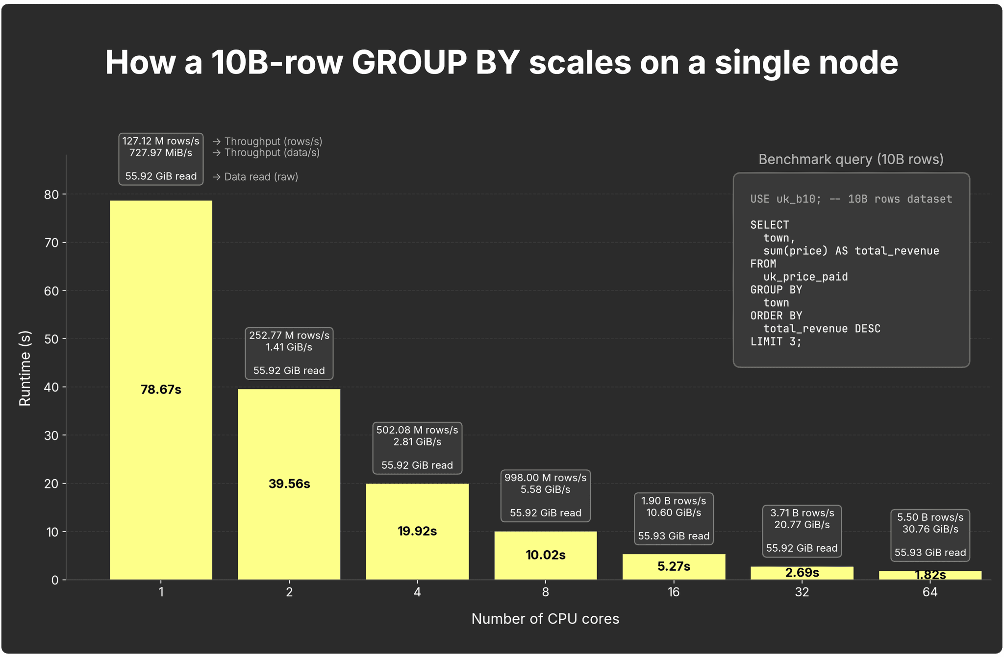
The chart below shows how our example GROUP BY query over 10 billion rows scales on a single node as cores increase:

Full results (plus detailed breakdowns of rows, bytes, and timings) are available in our benchmark GitHub repo here.

With 1 core, the query finishes in 78.7 s at ~127M rows/s (~728 MiB/s) end-to-end. Doubling cores nearly halves runtime and lifts throughput:

• 2 cores → 39.6 seconds, 253M rows/sec (~1.4 GiB/s)
• 4 cores → 19.9 seconds, 503M rows/sec (~2.8 GiB/s)
• 8 cores → 10.0 seconds, 998M rows/sec (~5.3 GiB/s)
• 16 cores → 5.3 seconds, 1.9B rows/sec (~10.6 GiB/s)
• 32 cores → 2.6 seconds, 3.7B rows/sec (~20.7 GiB/s)
• 64 cores → 1.9 seconds, 5.5B rows/sec (~30.6 GiB/s)

In short: GROUP BY scales almost linearly with cores. Each core builds partial states on its slice of the overall data; the engine merges them efficiently.

Where vertical scaling hits its limits #

This next query computes aggregates for every (county, town, district) in the 10B-row dataset:

• COUNT() – number of properties sold

• SUM(price) – total sales value

• AVG(price) – average sale price

It orders by total sales value and returns the top 10 areas or the most lucrative regions, respectively.

USE uk_b10; -- 10B rows dataset

SELECT
    county,
    town,
    district,
    formatReadableQuantity(count())    AS properties_sold,
    formatReadableQuantity(sum(price)) AS total_sales_value,
    formatReadableQuantity(avg(price)) AS average_sale_price
FROM uk_price_paid
GROUP BY
    county,
    town,
    district
ORDER BY sum(price) DESC
LIMIT 10
SETTINGS
enable_parallel_replicas = false;

On a maxed-out 89-core node, runtime was 14.4 s (~692M rows/s). Ok speed, but not interactive, 14 seconds feels long in dashboards or ad-hoc analysis.

About the time to tie your shoes, wait at a red light, or reheat a slice of pizza in the microwave.

For fixed cardinality workloads like this (the UK isn’t adding new counties or towns), an incremental materialized view is the obvious answer. Pre-aggregating by geography cuts data volume dramatically and guarantees millisecond response times.

Materialized views: storing partial states on disk
ClickHouse incremental materialized views extend the partial aggregation states idea: instead of recomputing GROUP BY at query time, they capture the partial aggregation states during inserts, store them in data parts, and let background merges incrementally combine them. Think of it as aggregation running continuously in background pipelines. We’ll explore this in detail in a follow-up.

But pre-aggregation isn’t always feasible. In observability, every log line counts, and ad-hoc queries may slice across any dimension. Same when grouping cardinality isn’t fixed. Then the alternative is brute force: When one big box, even with 89 cores, isn’t enough, the only option is to scale out. That’s where parallel replicas come in.

Scaling GROUP BY horizontally (with parallel replicas) #

Scaling out made simple: In ClickHouse Cloud, compute is decoupled from storage, so new compute nodes come online instantly.

Instead of physically sharding data, all nodes in ClickHouse Cloud read from a single limitless shard in object storage, acting as virtual replicas. With the parallel replicas feature, those nodes become additional parallel processing streams for the same query. More nodes → faster queries. A single coordinator orchestrates, dynamically slicing the data across nodes at runtime (think of it as virtual sharding on demand):

(The feature is currently in beta in ClickHouse Cloud; you can enable it today for some of your workloads, with GA coming soon.)

Without parallel replicas, a GROUP BY query could only use the cores of a single node (89 in our setup). With parallel replicas, every node’s cores join the same query:

• At the default 3 nodes, you already scale from 89 → 267 cores.

• At 10 nodes, that’s 890 cores.

• At 20 nodes, 1,780 cores.

• At 100+ nodes, you’re fanning a single GROUP BY across 8,900+ cores (and 35,600+ GiB RAM).

This is done without sharding or data movement, just by adding additional stateless compute nodes. It's one click (or API call).

In this post, we stop at 100 nodes; the “how far can it go?” exploration is something we’ll save for a dedicated follow-up once parallel replicas are GA.

Note: Parallel replicas also accelerate scalar aggregates and plain SELECTs: for scalar aggregates (e.g., SUM/AVG without GROUP BY), the compute nodes build, send, and merge the same partial states described above; for non-aggregate SELECTs, nodes process data in parallel and send sub-results, and the coordinator performs the final SORT/LIMIT.

How work is split across replicas #

The chart shows how our 10B-row GROUP BY scales across nodes (each with 89 cores):

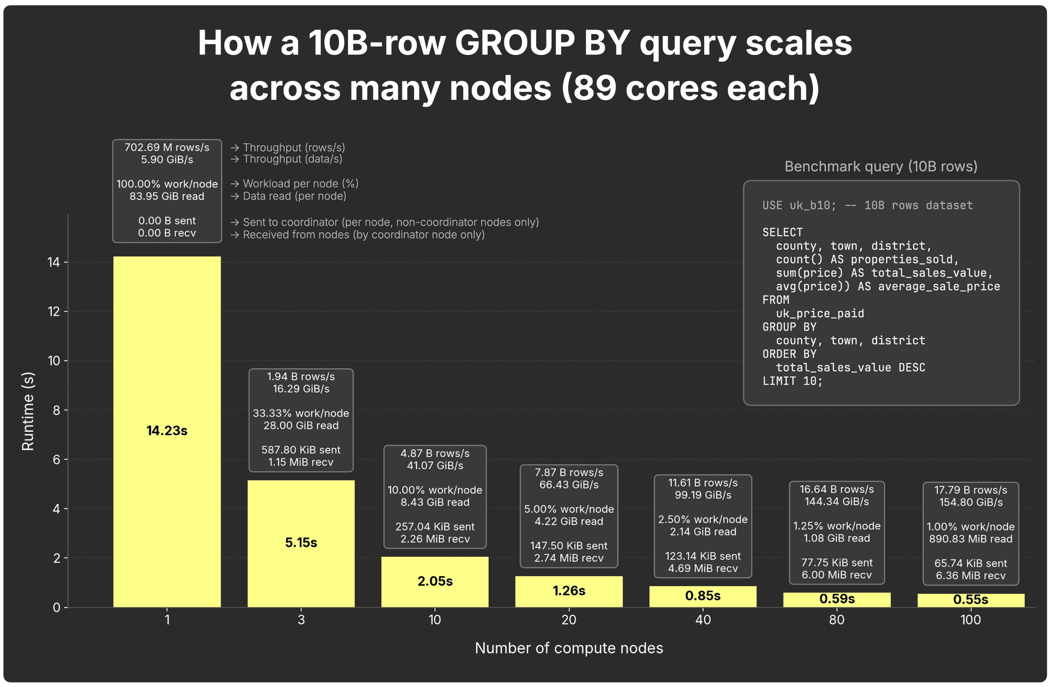
Here are the full results behind the chart above.

With 1 node, the query finishes in 14.2 s at ~703M rows/s (~5.9 GiB/s).

Adding additional nodes cuts runtime (and boosts throughput):

• 3 nodes → 5.2 s,
• 10 nodes → 2.0 s,
• 20 nodes → 1.3 s,
• 40 nodes → 0.85 s,
• 80 nodes → 0.56 s,
• 100 nodes → 0.55 s.

The chart also shows per-node workload participation, per-node data read (uncompressed), and network traffic (each node sends partial states to the coordinator, which receives them from all nodes and merges them).

Peeking behind the numbers: Our benchmark driver tracks way more detail: rows processed per node, compressed/uncompressed bytes scanned, memory usage, scan vs. aggregation time, cold/warm/hot status. We left that out to keep the charts clean, but the full results are in our GitHub repo.

Scaling isn’t perfectly linear, doubling nodes doesn’t always halve runtime, but it’s close. One node scans ~84 GiB; three nodes ~28 GiB; ten nodes ~8 GiB. At 80–100 nodes, each replica handles ~1 GiB or less, and coordination overhead (e.g., partial states sent over the network to the coordinator) starts to dominate, flattening the curve on smaller datasets.

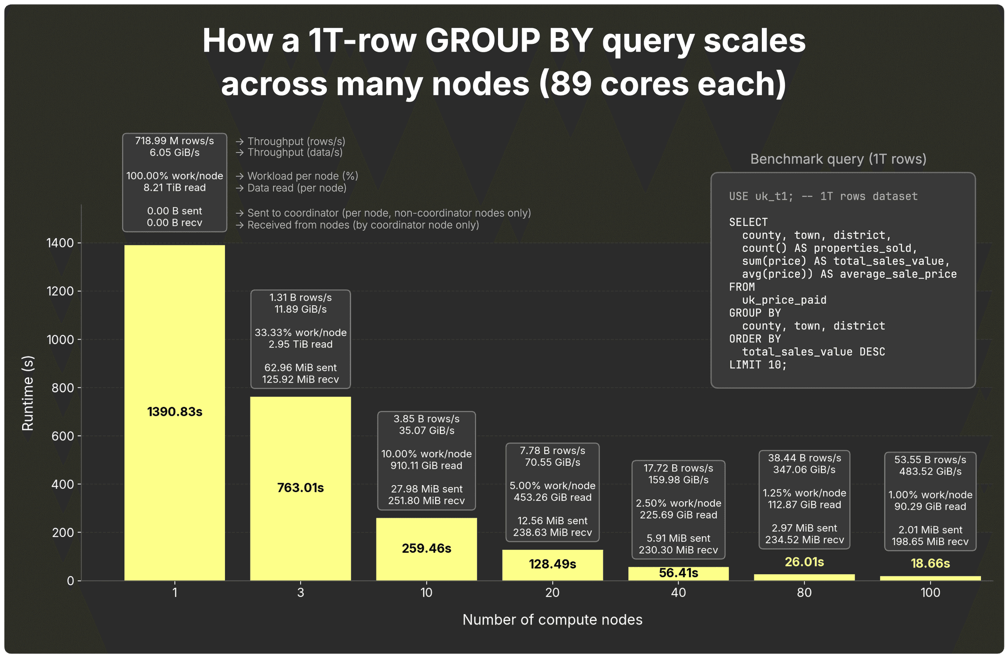
Scaling at 1T rows #

That flattening appears when per-node work gets too small to justify parallel replicas’ coordination overhead. To prove it, we reran the same query on the same compute nodes (each with 89 cores) on a dataset 100× larger: 1 trillion rows.

Full results are here.

At small node counts, each node is overloaded: a single node must scan and aggregate 8.2 TiB, and with 3 nodes it’s still nearly 3 TiB each.

With 10 nodes the per-node read drops to ~910 GiB, and scaling kicks in nicely. Then node doublings are linear or better:

• 10 → 20 nodes: 2.02× faster
• 20 → 40 nodes: 2.28× faster
• 40 → 80 nodes: 2.17× faster
• 80 → 100 nodes: 1.39× faster (better than the linear 1.25× expectation)

Even at 100 nodes, each replica processes ~90 GiB, which is enough work to justify the coordination overhead of parallel replicas, so scaling remains strong.

And yes, scaling would continue beyond 100 nodes on the 1T-row dataset, but as noted earlier, we’re saving the “how far can it go?” deep dive for a dedicated follow-up once parallel replicas are GA.

How well the parallel replicas feature works also depends on partial-state size; we’ll look at that next.

When GROUP BY gets heavy #

Not all GROUP BYs are created equal. So far, we’ve shown light aggregates like SUM and AVG, where partial states are tiny. But what happens when GROUP BY gets heavier, like COUNT DISTINCT? That’s where scaling looks different, and partial state size starts to matter.

To demonstrate this, we count distinct streets with sales in each county per quarter over the 10B rows dataset.

USE uk_b10; -- 10B rows dataset

SELECT
  county,
  toStartOfQuarter(date) AS qtr,
  uniq(street) AS distinct_streets_with_sales
FROM
  uk_price_paid
GROUP BY
  county, qtr
ORDER BY
  qtr, county;

The query is simple; the aggregate choice matters.

Note: This benchmark focuses on how different aggregate functions produce different partial state sizes. Since it uses a fresh GROUP BY query (different from earlier benchmarks), we ran it on 16-core nodes instead of 89-core ones, showing at the same time that parallel replicas scale efficiently regardless of core count.

The light case: uniq() #

uniq() is approximate but efficient. It uses adaptive sampling (up to 65,536 hashes), keeping states compact.

For full results, go here.

• Per-node sent states: ~58 MiB per sending node (2 senders with 3 nodes) to ~4.2 MiB per node with 100 nodes

• Coordinator received total: ~115 MiB (2×58 MiB) with 3 nodes to ~416 MiB (99x4.2 MiB) with 100 nodes

→ Coordinator fan-in stays small; per-node traffic shrinks as nodes increase.

The heavy case: uniqExact() #

uniqExact() computes true COUNT DISTINCT. Partial states grow because each node must track all distinct values it sees, stored either as raw values or as hashes, depending on type, before the coordinator merges them.

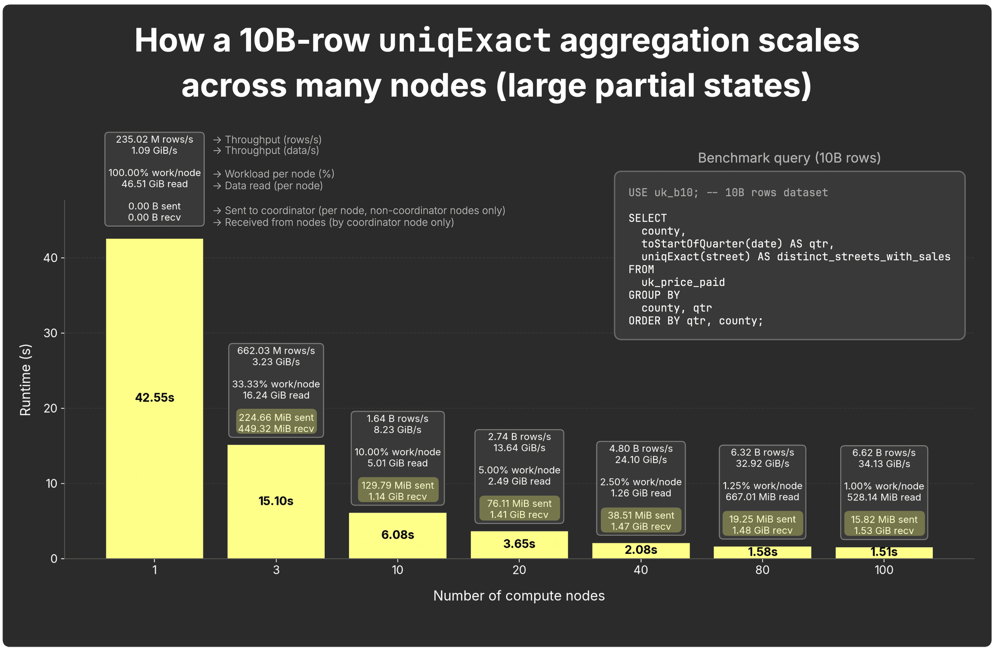
You find the full results here.

• Per-node sent states: ~225 MiB per sending node (2 senders with 3 nodes) to ~16 MiB per node with 100 nodes

• Coordinator received total: ~450 MiB (2×225 MiB) with 3 nodes to ~1.5 GiB (99x16 MiB) with 100 nodes

States are ~4× larger than with uniq(), so network fan-in and merge time are more noticeable, even though runtime still improves.

But this isn’t universal: uniqExact() state size scales with cardinality. In our data, unique streets per (county, quarter) max at ~17k and stay stable, making this example relatively mild.

Cardinality caveat: When distincts explode (e.g., uniqExact(user_id) for billions of users, or uniqExact(url) across the web), states can be orders of magnitude larger than uniq(), and network overhead grows accordingly.

Takeaways on distincts #

Parallel replicas scale all 170+ aggregate functions, but the size of partial states determines efficiency:

• Light states (e.g. sum(), count(), uniq()): scale well.

• Heavy states (uniqExact()): scale too, but with more network/merge cost.

• Other options (uniqHLL12()): fixed ~2.5 KB state with ~1–2% error for 10K–100M distincts; less accurate on tiny sets, degrades beyond 100M; a practical balance for some workloads.

Heavy aggregates still scale, but larger partial states increase network traffic and merge cost. Whether the trade-off pays off depends on how much data each node has to process. That brings us to the safeguards ClickHouse applies to keep parallel replicas efficient.

Scaling limits and safeguards #

One query doesn’t always get faster by throwing more nodes at it.

On smaller datasets (e.g., 10B rows), parallel replicas scale well at low node counts, but at higher counts, nodes may run out of work, and coordination overhead dominates.

On larger datasets (e.g., 1T rows), the opposite happens: low node counts can be overwhelmed, while higher counts scale cleanly because each node still has plenty of rows to process, making the coordination cost worth it.

ClickHouse uses two guardrails to keep parallel replicas efficient:

• parallel_replicas_min_number_of_rows_per_replica — only turns a node into a parallel replica if it gets enough rows to justify the overhead.

• max_parallel_replicas — caps the maximum number of nodes that are used as parallel replicas for a query (default 1000).

Behind the scenes, the query planner estimates rows_to_read (e.g., via index analysis), the number of rows it expects the query will actually scan and process. The two settings from above then decide together whether parallel replicas are worth it and, if so, how many to use:

• Enable rule: Parallel replicas are only enabled for a query if

rows_to_read >= 2* parallel_replicas_min_number_of_rows_per_replica

Otherwise, they’re disabled, and the query runs on a single node.

• Limit rule: If enabled via rule above, the number of nodes used as parallel replicas (number_of_replicas_to_use) is limited to

rows_to_read / parallel_replicas_min_number_of_rows_per_replica

(still capped by min(cluster size, max_parallel_replicas))

If this value is ≤ 1, parallel replicas are also disabled and the query falls back to normal single-node execution.

In other words: small datasets skip parallel replicas entirely; large ones use them, but only up to the point where each node still gets meaningful work.

Example: Say a query has 10B rows to read, max_parallel_replicas = 100, and parallel_replicas_min_number_of_rows_per_replica = 1B.

• Enable rule: 10B ≥ 2×1B → passes (parallel replicas enabled).

• Limit rule: 10B ÷ 1B = 10 → 10 nodes used as parallel replicas for the query (not 100).

Each activated node then processes ~1B rows, enough work to justify the overhead.

Default behavior: By default, parallel_replicas_min_number_of_rows_per_replica is 0, which disables this safeguard. In that case, parallel replicas are always enabled, capped by max_parallel_replicas (default 1000) or by the cluster size, whichever is smaller. On small datasets, this can add unnecessary coordination overhead, so tuning the setting is recommended in production. You can also toggle parallel replicas per query with enable_parallel_replicas, and, if needed, override max_parallel_replicas for that query.

Together, these safeguards try to ensure parallel replicas only kick in when they’ll cut query time, not add to it.

Next, let’s look under the hood at how parallel replicas actually distribute work across nodes.

How parallel replicas distribute work #

(We’ve already published a detailed guide on how work is distributed with parallel replicas; here we’ll just summarize the essentials.)

The node that receives a query (in ClickHouse Cloud, the one picked by the load balancer) always becomes the coordinator for that query. Importantly, the coordinator is also a full parallel replica, executing its share of work just like the others, as shown in the earlier animation.

Once a query arrives, the coordinator plans the work in ranges of granules (the smallest unit of processing in ClickHouse, ~8,192 consecutive rows by default, selected via index analysis). It assigns granules across participating replicas, including itself.

Each replica scans its assigned granules locally, computes partial aggregation states, and streams those states back. The coordinator then performs the final merge and returns the result.

This granule-based model enables fine-grained load balancing:

• Dynamic coordination: replicas request new tasks as they finish previous ones, so faster replicas automatically pick up more work.

• Task stealing: if one replica lags, others can grab its remaining granules.

• Cache locality: Via consistent hashing, the same nodes process the same granules on repeated queries, reusing cached data. This works best when the full cluster is used (cluster size ≤ max_parallel_replicas); otherwise, node assignment is random.

That’s enough ground-level detail. Time to take a bird’s-eye view and see how GROUP BY has evolved in the broader perspective of our cloud.

GROUP BY at cloud scale #

In ClickHouse Cloud, GROUP BY now scales elastically across fleets of nodes in two complementary ways:

• Inter-query scaling: add more nodes, and you can run more queries at once. The load balancer simply has a larger compute pool to route requests to, so overall throughput rises with cluster size.

• Intra-query scaling (focus of this blog): make one query faster by splitting it across many nodes. With the parallel replicas feature enabled, ClickHouse parallelizes queries across all available CPU cores of all available nodes.

In open-source ClickHouse, a single query can also scale with sharding or parallel replicas. Sharding spreads data across nodes but requires resharding to add capacity, potentially hours or days of work. Parallel replicas work too, but in shared-nothing setups, they need full physical copies of the data.

In the cloud, the model shines brighter: compute is decoupled from storage, and each node is effectively a stateless virtual replica reading from shared object storage. Nodes can be added or removed instantly, with no data copying or reshuffling, and single-query speedups come with a flip of a switch.

The cloud adds even more lift. A distributed cache keeps hot data close to compute nodes, accelerating repeated queries across the fleet. A Shared Catalog centralizes database metadata so new nodes come online in moments, and GROUP BY also works seamlessly over open table formats like Iceberg and Delta Lake alongside native tables.

Queries over external formats use the same partial-aggregation-state execution model we’ve explored in this post. With native tables, parallel replicas split work by granule. With external formats, you need to use …Cluster functions—like s3Cluster, azureBlobStorageCluster, deltaLakeCluster, icebergCluster, and more—which split work by file (e.g. Parquet files in Iceberg).

In other words, whether data lives in native tables or external in open formats, ClickHouse Cloud can fan out a GROUP BY across its stateless compute nodes and still deliver results at interactive speed.

From one node to the cloud #

This post has been my own journey, from disbelief at a single-node query finishing faster than a blink, to watching the same model stretch seamlessly across fleets of machines.

GROUP BY sits at the core of nearly every analytical query: powering observability dashboards, fueling conversation-speed AI, agent-facing analytics, and everything in between.

ClickHouse was built to run GROUP BY fast. In the cloud, that design evolved into something even more powerful: with parallel replicas, the processing-stream-per-core model scales elastically across all cores of all nodes, giving you interactive speed on data of any shape and scale.

The elegance is its simplicity: partial states per processing stream, merged into correct results at any scale.

Just like the fountain pen, ClickHouse still does one thing exceptionally well: GROUP BY, only now at a scale and speed that stretches seamlessly from your laptop to the cloud.

Parallel replicas are in beta today and will soon be generally available in ClickHouse Cloud. You can already enable them for some of your workloads to experience these speedups firsthand.