TL;DR
Agentic workloads put continuous pressure on analytical systems, and the ability to keep fresh data query-ready becomes a cost issue.
ClickHouse obtains query-ready data at 22× lower cost and delivers 28× better write-side cost-performance, using Snowflake as a measured contrast point.
This is the write side of cost-performance, and it is rarely measured directly.
For the complete picture, see our companion blog that measures the full real-time analytics path, from ingestion through query execution.
Agentic analytics starts before the query
Most cloud data warehouse benchmarks start when the query begins.
That makes sense for traditional analytics. A human analyst opens a dashboard, writes a SQL query, waits for a result, and maybe asks a follow-up. In that world, measuring query runtime and query cost tells most of the story.
Agentic analytics changes the shape of the workload.
A single user question can turn into dozens of SQL queries: schema exploration, candidate query generation, validation queries, retries, refinements, drilldowns, and follow-up analysis.
Those queries sit on the critical path of the user experience: if the database is slow, a chat with an agent feels slow. For autonomous agents, the pressure is even higher: without human input latency, each loop is limited mostly by LLM latency and data retrieval latency. That makes low-latency answers over fresh, often-changing data essential.
Multiply that across users and agents, and the warehouse no longer sees occasional queries, but bursts of concurrent analytical queries, each with low-latency expectations.
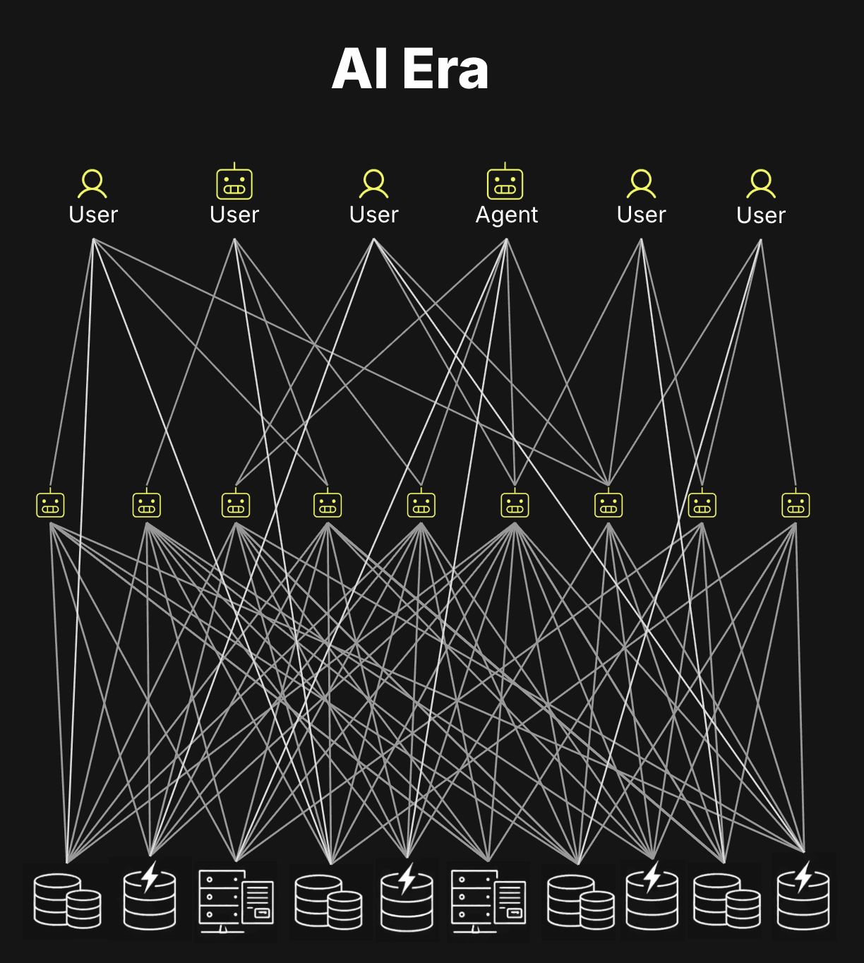
This is the shift described in our earlier post on how AI is redrawing the database market: agent-facing analytics makes internal analytical workloads look more like customer-facing applications - high-concurrency, low-latency, and interactive.
Those queries increasingly run against fresh data.
New events keep arriving. Tables keep growing. Agents keep asking. The data has to stay query-ready as it changes.
That means query cost-performance starts before the query.
Before a query can be fast, newly ingested data has to be written, ordered, compressed, and prepared for pruning.
If the storage layer does this efficiently, queries can skip more data and stay cheap. If it does this inefficiently, the system either spends more compute in the background, reads more data at query time, or both.
This is the write side of cost-performance, and it is rarely measured directly.
So we move the benchmark boundary from the first query to the first write.
The core question is how efficiently a system can keep fresh data query-ready in real time.
We use Snowflake as the contrast point because it represents the opposite end of the architectural spectrum: data is written first, then clustered later to establish locality, allowing queries to skip more data. ClickHouse takes the other path: it creates that ordered layout as part of the write path and preserves it through the storage engine as data grows.
What about BigQuery, Databricks, and Redshift? (click to expand)
A full write-side cost-performance benchmark across all major cloud data warehouses is outside the scope of this post. We focus on Snowflake and ClickHouse because they represent two ends of the architectural spectrum: Snowflake establishes ordering after the write, while ClickHouse builds it into the write path. The other major cloud warehouses fall between these poles, but none cross to ClickHouse's side.
BigQuery writes data into sorted storage blocks on arrival, but new inserts create overlapping ranges that require automatic background reclustering to restore order. That reclustering is free - Google absorbs it into the platform - but data written since the last recluster is not yet fully organized for pruning.
Databricks SQL Serverless sits closest to Snowflake. Data lands in Parquet files in arrival order. Liquid Clustering reorganizes them post-ingest via an OPTIMIZE job, which runs on separate serverless compute and is billed as such.
Redshift sorts data post-ingest using a background process that runs on the provisioned cluster itself. There is no separate clustering service or charge, but new rows land unsorted and stay that way until the background sort reaches them.
The pattern is similar: keeping data organized for pruning is work. Depending on the system, that work may show up as a separate charge, run on provisioned compute, or be absorbed into the platform - but it still affects the economics of keeping fresh data query-ready.
To make that difference concrete, we measure the cost of keeping the same dataset query-ready for fast analytics while continuously ingesting roughly 1 million rows per second, and show why the write path becomes part of the cost-performance equation.
That raises the first question: what does “query-ready” actually mean?
What does “query-ready” mean?
For an analytical query, query-ready data means the engine can avoid reading most of the table.
The fastest analytical queries are the ones that read the least data.
Analytical workloads typically filter contiguous ranges of rows, for example all events for a specific day in a web analytics table, and then aggregate the results, as in the query below:
SELECT
    URL,
    COUNT(*) AS pageviews,
    COUNT(DISTINCT User) AS users
FROM hits
WHERE Day = 'D2'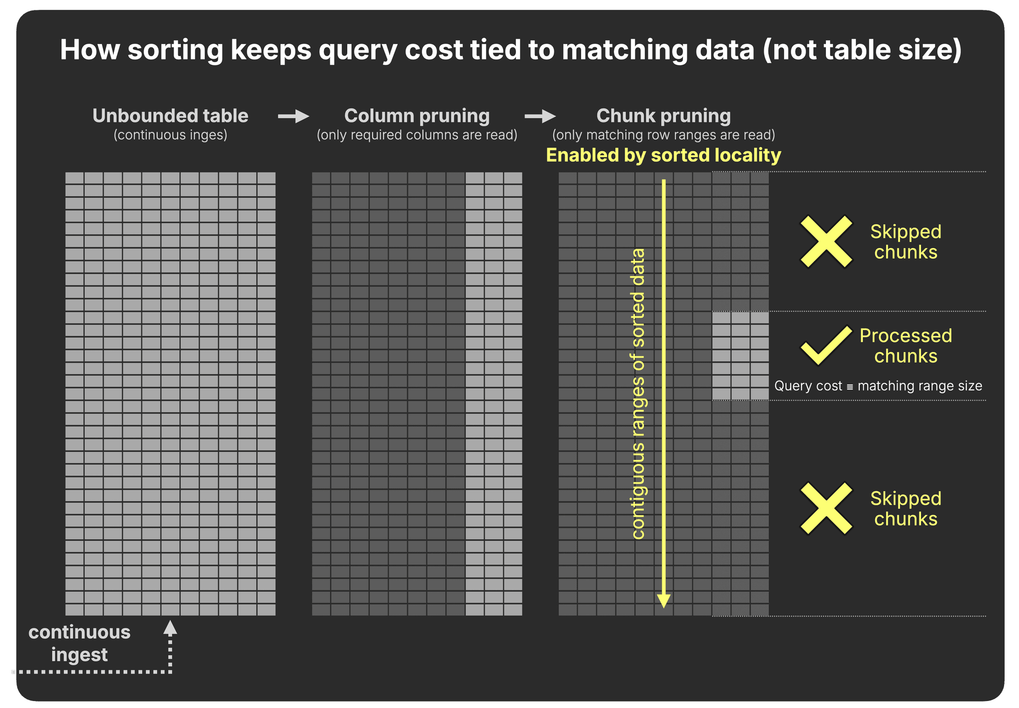
GROUP BY URL;To execute such queries efficiently, analytical databases rely on two core ideas.
First, columnar storage enables pruning at the column level: although the table may contain hundreds of columns, this query touches only Day, User, and URL, all other columns are skipped.
Second, data is processed in chunks, not rows. This enables pruning at the chunk level: entire blocks of rows are either read or skipped.
Together, these mechanisms reduce I/O and enable efficient vectorized execution.
However, pruning at the chunk level is only effective when the data is stored sorted on the filtered column. If the table is unsorted, chunks will typically contain mixed values:
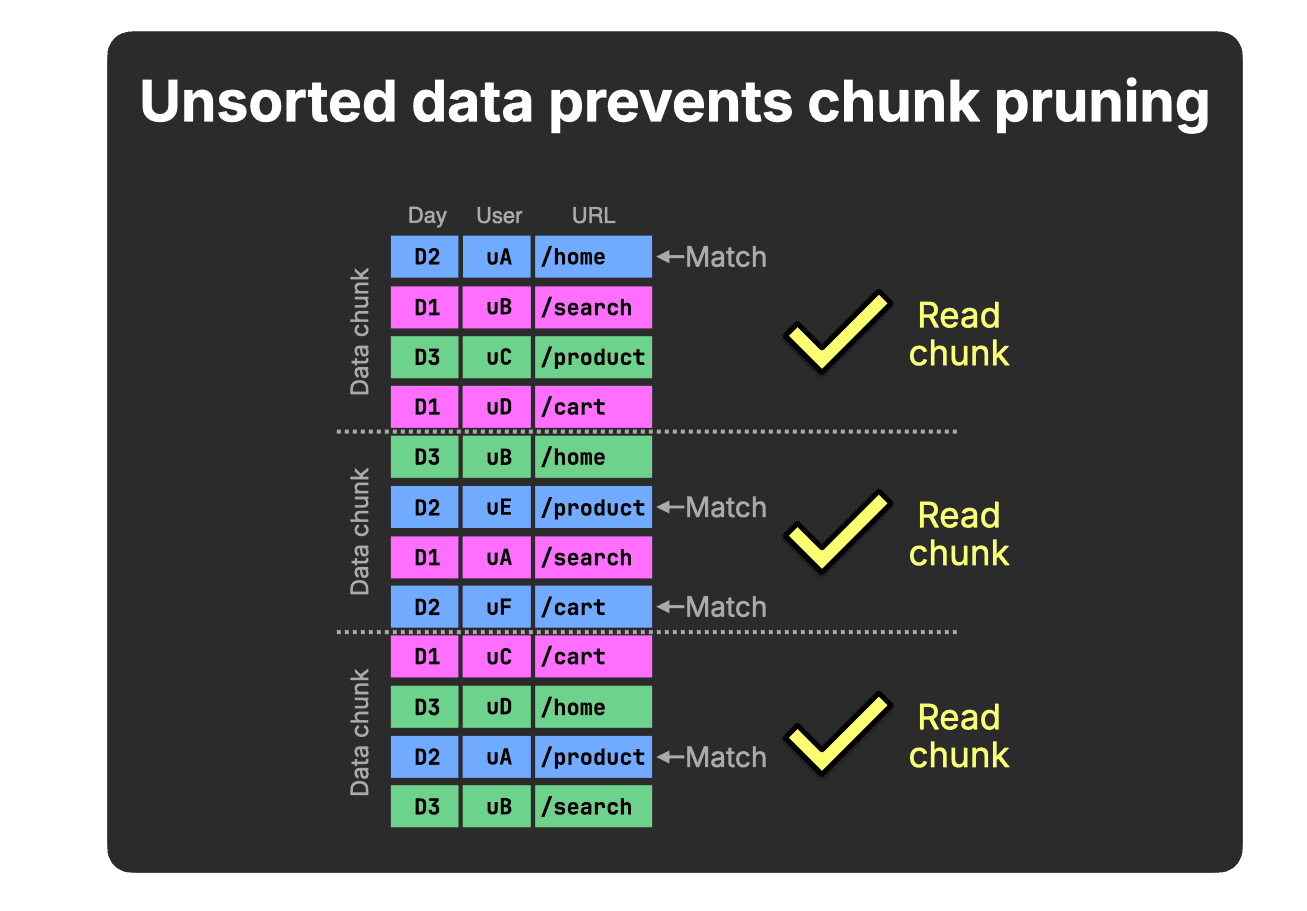
In this simplified example (four rows per chunk), each chunk contains at least one D2 value, therefore, none can be skipped for our query’s Day = D2 predicate.
When related Day rows are stored contiguously, value ranges within chunks no longer overlap, and non-matching chunks (for our query’s Day = D2 predicate) can be skipped entirely:
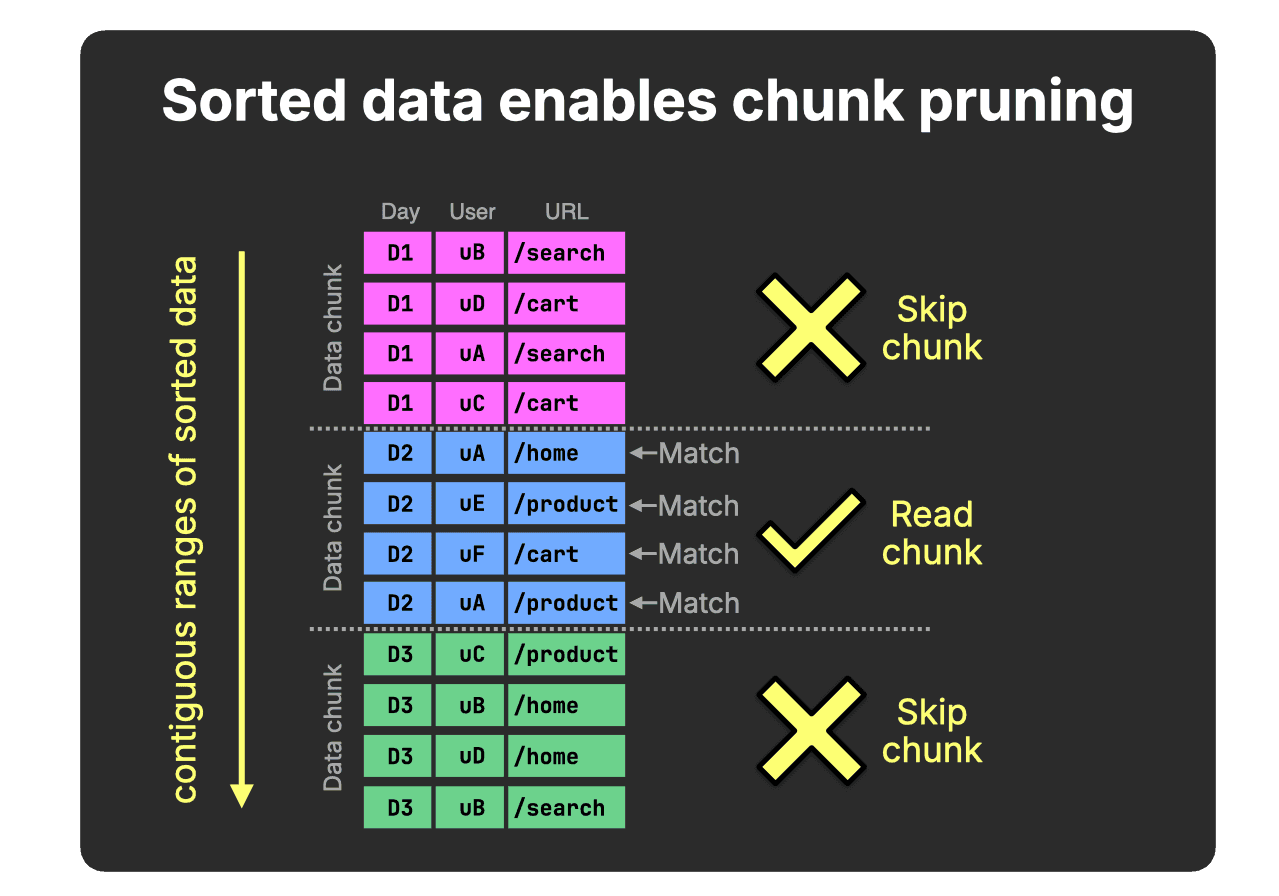
Sorting tightens value ranges within chunks and enables effective pruning.
This is the structural requirement that allows analytical queries to skip large portions of the table, even before additional optimizations like pre-aggregation are applied.
Why not rely on materialized views? (click to expand)
Materialized views are another common technique to accelerate analytics by pre-aggregating data, reducing how much raw data must be scanned.
However, raw tables still need to support ad-hoc queries, debugging, new query patterns, joins, drill-downs, and observability queries that were not anticipated when the views were created.
Efficient data ordering therefore remains critical for scalable analytics, even in systems that use materialized views.
This applies to the materialized views themselves as well: at scale, ordering still determines whether queries can skip most of the materialized view’s data.
Additional techniques, such as lightweight projections, can further accelerate queries whose filters do not align with the primary ordering.
Ultimately, the same rule still holds:
Skipping data is the only way analytics scales.
Sorting is the primary mechanism that enables skipping.
And at first glance, Snowflake and ClickHouse Cloud look strikingly similar here: both rely on columnar storage and chunk-level pruning to avoid scanning unnecessary data, which in turn depends on how related rows are physically organized.
Pruning must survive continuous ingest
In modern real-time analytics, data is not written once and queried many times.
Tables grow continuously as new data keeps arriving.
Under that regime, keeping data continuously sorted ensures that query cost depends on what matches, not on the total data stored.
What matters, then, is when and how sorted locality - rows with similar key values stored contiguously - is created and maintained as new data keeps arriving.
In a world of continuous ingest, how a warehouse organizes data after it is written determines how efficiently it scales.
We now examine how Snowflake and ClickHouse create and maintain that locality under continuous ingest.
Get started today
Interested in seeing how ClickHouse works on your data? Get started with ClickHouse Cloud in minutes and receive $300 in free credits.
Sign upTwo ways to obtain query-ready data
The key difference is when locality is created: after data is written, or while it is being written.
Snowflake: clustering after ingest
Snowflake’s prunable data chunk is the micro-partition, an immutable compressed columnar unit.
Each micro-partition typically stores ~50–500 MB of data (before compression) and includes per-column min/max statistics used for pruning.
Each INSERT creates a new micro-partition.
Data is written in arrival order, as illustrated below with three example inserts:
(In the animation above, for clarity, we show the min..max values only for the Day column, but they are created for all columns.)
Data is not automatically sorted.
Under continuous ingest, the absence of sorted locality becomes costly.
Every insert produces another independently written micro-partition. Over time, value ranges overlap across partitions. When filtering on a column like Day, many partitions contain mixed values, and therefore cannot be skipped:
Because the Day ranges overlap across partitions, pruning via min/max metadata is ineffective for this predicate.
A note on pre-sorting in Snowflake (click to expand)
Pre-sorting input data may reduce value-range overlap within a single insert batch.
However, each INSERT still creates independent micro-partitions.
Over time, ranges across partitions will overlap again.
To establish sorted locality, Snowflake provides clustering.
When a clustering key is defined (the Day column in our example), Snowflake rewrites existing micro-partitions in the background, replacing them with newly organized ones that group similar key values together. This tightens min/max ranges and enables effective pruning:
After clustering, micro-partitions contain narrower value ranges, and non-matching partitions can be skipped entirely:
In Snowflake, sorted locality is not created at write time. It is established later by rewriting data after ingestion.
Under continuous ingest, clustering must run continuously to re-establish sorted locality.
What about observability data, where events arrive in timestamp order? (click to expand)
A reasonable objection: if observability events arrive roughly in ingestion order, each new micro-partition gets a non-overlapping timestamp range, and min/max pruning on the timestamp column works without clustering. That is partially correct - for a pure timestamp-only workload with perfectly ordered ingest.
In practice, this breaks down on multiple fronts. First, real observability pipelines are not perfectly ordered: distributed collectors buffer and flush independently, Kafka consumers lag and catch up, retries produce late-arriving events, and cross-service clock skew is routine. Even occasional overlap reintroduces the partition-scanning problem and triggers the clustering service.
Second, and more fundamentally, observability queries are rarely single-dimensional on timestamp.
The typical query is WHERE service = 'checkout' AND timestamp > now() - interval 1 hour,
or filters on trace_id, error_level, or span_id.
Arrival-order storage leaves all of those dimensions completely unordered - pruning on them
is just as ineffective as in the general case, regardless of how neatly the timestamps arrived.
Third, Snowflake's own documentation warns that high-cardinality timestamp columns make poor clustering keys directly. The recommended workaround - casting to date - reduces pruning granularity to the day level, which is too coarse for the sub-hour queries common in observability.
Re-establishing sorted locality is one approach. Preserving it is another.
ClickHouse: ordering on the write path
ClickHouse’s prunable data chunk is the granule.
A granule typically contains ~8K rows or ~10 MB of data (before compression) and is a logical unit within an immutable, sorted data part.
Unlike Snowflake, sorted locality is created as part of the write path.
Each INSERT produces a new data part that is already sorted by the table’s sorting key (the Day column in our example), as illustrated below with three inserts:
Because data is automatically written sorted, contiguous key ranges are established immediately. The sparse primary index records range boundaries at the granule level (8,192 rows per granule by default; 2 rows in our example), enabling highly granular pruning during query execution.
Isn’t write-time sorting expensive? (click to expand)
Although sorting may appear costly, in practice it is highly efficient.
Inserts are already processed in memory in columnar blocks, and sorting by the sorting key is a parallel, cache-efficient step.
In our ingestion benchmarks, server-side sorting overhead was negligible compared to parsing and network transfer.
This achieves the same outcome as Snowflake’s min/max metadata: entire chunks can be skipped based on value ranges.
The difference appears in what happens next.
Under continuous ingest, preserving this locality becomes critical.
As new parts keep arriving, the engine continuously merges smaller parts into larger ones in the background:
Because all parts are already sorted by the same key, the engine performs a single linear merge pass with no re-sorting required.
Why ClickHouse merges are CPU-efficient (click to expand)
ClickHouse can merge parts efficiently because all parts are already sorted by the same key.
When parts are merged, the engine performs a single linear merge pass, similar to the merge step of merge sort:
- parts are read sequentially
- rows are compared on the fly
- a new merged part is written out
No re-sorting, random access, or large temporary buffers are required.
Because merges operate on already sorted streams, they are largely sequential and cache-efficient.
This mechanism allows ClickHouse to continuously consolidate data in the background while preserving sorted locality.
With each merge, similar sorting key values become increasingly co-located. This tightens the value ranges recorded in the sparse primary index, allowing entire granules to be skipped for predicates on the sorting key, as illustrated below.
At query time, this achieves the same range-pruning effect as Snowflake’s clustering.
The difference is that in ClickHouse the mechanism is built directly into the storage engine rather than applied afterward.
How this compares to Snowflake at query time (click to expand)
At query time, there is no fundamental difference in how pruning works.
Both Snowflake and ClickHouse use range metadata to skip large chunks of data:
- Snowflake stores explicit min/max statistics per micro-partition (~50–500 MB before compression).
- ClickHouse stores the first sorting-key value per granule (~10 MB before compression) in its sparse primary index.
This allows ClickHouse to prune at significantly finer granularity.
Because ClickHouse data is physically sorted on the sorting key:
- Each granule implicitly defines a contiguous value range.
- The first value of the next granule effectively acts as the upper bound of the previous one.
Conceptually, this achieves the same outcome as Snowflake’s min/max metadata: entire chunks can be eliminated based on value ranges. The difference is not in how pruning works but in how those value ranges are created and maintained over time.
In ClickHouse, ordering is built into the storage engine by design.
With each merge, sorted segments grow larger, and under continuous ingest, that structural consolidation compounds.
Under continuous ingest, ordering mechanics become economics.
Measuring the cost of query-ready data
This benchmark extends our previous read-side cost-performance study, which measured query runtime and compute cost of analytical queries across five cloud data warehouses on the same production-derived, anonymized ClickBench web analytics dataset.
Note that this is a controlled experiment, not an ingest speed comparison. We ingest the ClickBench dataset with a modest 1 million rows per second rate - well within the operational range of both systems - and measure the compute cost of keeping that continuously ingested data organized for fast analytical queries. The same pricing methodology from our previous cost-performance study is applied throughout, and the read benchmark uses the same 43 ClickBench queries. All benchmark code and raw results are published on GitHub.
How we ingested 1 million rows per second (click to expand)
Snowflake was loaded via a single continuous stream into the table, using a Gen1 M warehouse.
ClickHouse was loaded via a Python script
using the ClickHouse Connect
client, simulating 170 parallel clients each sending a
continuous stream of 20,000-row batches. This uses
async inserts
- now the default ingest mode
in ClickHouse - which buffer rows server-side before flushing a sorted part, allowing
high client concurrency without causing part explosion. With a 2 GB buffer per node and
3 nodes, each buffer flushed roughly every 3 seconds -
measured via part_log system table (avg: 2.91s).
Both systems organize the data on the identical key: Snowflake through a clustering key, ClickHouse through a sorting key.
Isolating the cost of ordered data
Because both systems offer compute-compute separation, we can precisely measure the cost of obtaining ordered data, separate from the cost of querying it.
We’ll start with two high-level animations showing how we configured each system to isolate write and ordering compute from read compute, and the costs that fall out of that setup.
Snowflake benchmark setup: writes, clustering, reads
The Snowflake setup separates the workload into three compute surfaces: a write warehouse, a managed clustering service, and a read warehouse.
① Writes in arrival order
As explained earlier, Snowflake writes incoming rows in arrival order into micro-partitions.
For our sustained ingest workload, a Gen1 M warehouse was sufficient to ingest 1 million events per second. At Enterprise pricing, this costs $336 per 100B rows of ClickBench data.
② Background clustering
Ordering happens later.
To keep the table clustered for fast analytics, Snowflake uses automatic clustering: a managed background service that rewrites micro-partitions outside the write warehouse.
In our run, this added roughly $2,500 per 100B rows. Users do not directly control how much compute automatic clustering uses or how long reclustering takes.
③ Range pruning
The read benchmark runs separately, after the data has been clustered.
A Gen2 4XL warehouse completed the 43 ClickBench queries over 100B ordered rows in 176 seconds, at an Enterprise-tier compute cost of $25.
ClickHouse uses the same benchmark split, but the write-side work is different: writes and ordering happen together.
ClickHouse benchmark setup: writes and ordering, reads
① Write-time ordering
As mentioned in the previous section, in ClickHouse, incoming rows are written into sorted data parts, so contiguous key ranges are established immediately. In our setup, a 3-node write & ordering service with 8 CPU cores and 32 GiB RAM per node sustained 1 million events per second.
At Enterprise pricing, this costs $131 per 100B rows of ClickBench data - 95% less than Snowflake’s combined write and clustering cost for the same workload.
② Order-preserving background merges
Ordering is preserved by background merges running on the same provisioned service.
As a reminder, these merges combine smaller sorted parts into larger sorted parts. As the parts grow, key ranges become more contiguous, compression improves, and the amount of data future queries need to read goes down.
There is no separate clustering service and no separate clustering charge.
③ Range pruning
The read benchmark runs separately, against the ordered data.
A 40-node read service completed the 43 ClickBench queries over 100B ordered rows in 126 seconds, at an Enterprise-tier compute cost of $16 - 28% faster and 36% cheaper than Snowflake on the same ordered dataset.
The ClickHouse setup only works if the write & ordering service can keep up with ingest. The dashboard below shows that it did.
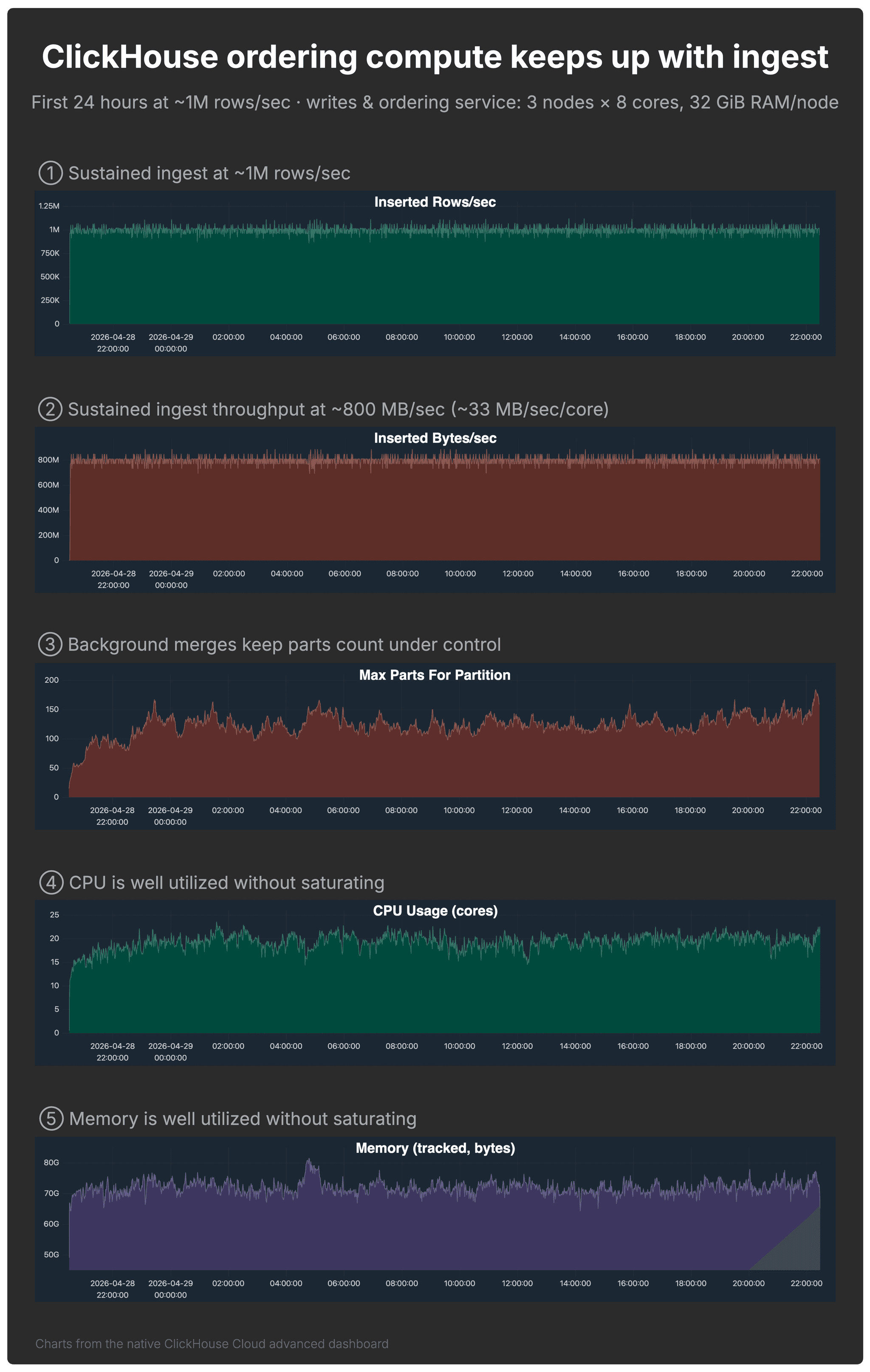
ClickHouse write & ordering compute keeps up with ingest
The 3-node ClickHouse write & ordering service with 8 CPU cores and 32 GiB RAM per node sustained the workload while keeping the table query-ready.
The charts below, from the native ClickHouse Cloud advanced dashboard, show the first 24 hours of the run and validate the setup from several angles.
- ① Rows/sec: ingest stayed around 1 million rows per second.
- ② Bytes/sec: ingest also stayed around 800 MB/sec, or roughly 33 MB/sec per CPU core. This matters because rows/sec alone can be misleading: 100 million tiny rows/sec is not necessarily more demanding than 1 million wide rows/sec. The bytes/sec chart gives a better sense of the actual write throughput the service sustained.
- ③ Part count: background merges kept the maximum part count in the single default partition under control. The table was not explicitly partitioned.
- ④–⑤ CPU and memory: both were well utilized without saturating.
What about Snowflake CPU and memory metrics? (click to expand)
For ClickHouse, we show CPU and memory from the native ClickHouse Cloud advanced dashboard because the write & ordering service exposes resource utilization directly.
Snowflake exposes warehouse load, query history, query profiles, and credit usage, but not an equivalent native node-level CPU and memory dashboard for a virtual warehouse.
So for Snowflake, we validate the setup by outcome and cost: the write warehouse sustained the same 1 million rows per second ingest rate, and the consumed warehouse credits capture the cost. A comparable CPU/memory saturation chart is not available through Snowflake’s native observability surface.
With ingest, part counts, CPU, and memory all under control, the important question becomes when fresh data is actually ready for efficient queries.
Query-ready immediately vs. waiting for clustering
Both systems aim for the same outcome: ordered data that can be pruned efficiently. The difference is when fresh data reaches that state.
ClickHouse does not wait for a background process to make fresh data useful
Write-time ordering enables immediate range pruning, while background merges incrementally improve the layout over time. In the part-count chart above, the maximum stays roughly between 100 and 150 parts per partition, showing a healthy, query-efficient layout for this workload at each point in time - because ingest is continuous, merges are never “finished” - and they do not need to be. Queries benefit from ordering immediately; merges simply improve that layout over time.
Snowflake has a different dependency: clustering has to catch up
After the first 100B rows, the table contained roughly 540K micro-partitions. Starting from an empty table, automatic clustering began 1.3 hours after ingest started and finished 6.7 hours after the 100 billionth row was ingested.
That lag matters for real-time analytics: fresh data may be present in the table before it is fully organized for fast pruning.
Alternative to automatic clustering (click to expand)
As an alternative to automatic clustering, Snowflake users can manually rewrite tables, for example via
CREATE TABLE sorted_table AS SELECT * FROM unsorted_table ORDER BY sorting_column.
This rewrite runs on warehouse compute, processes the full dataset, and does not provide incremental locality maintenance. Under continuous ingest, the rewrite must be repeated, turning it into an ongoing task.
This approach can work for periodic batch refreshes, but becomes operationally heavy for continuously growing tables.
The setup above gives us all the pieces. Now we combine the write and ordering costs across the 100B, 200B, and 300B row checkpoints.
The cost of obtaining query-ready data
Based on the setups shown by the two animations above, the chart below shows the cumulative compute cost of obtaining ordered data for fast analytics at 100B, 200B, and 300B rows.
Both systems continuously ingest the ClickBench dataset at 1 million rows per second and organize it on the same key: Snowflake through clustering, ClickHouse through write-time ordering and order-preserving background merges.
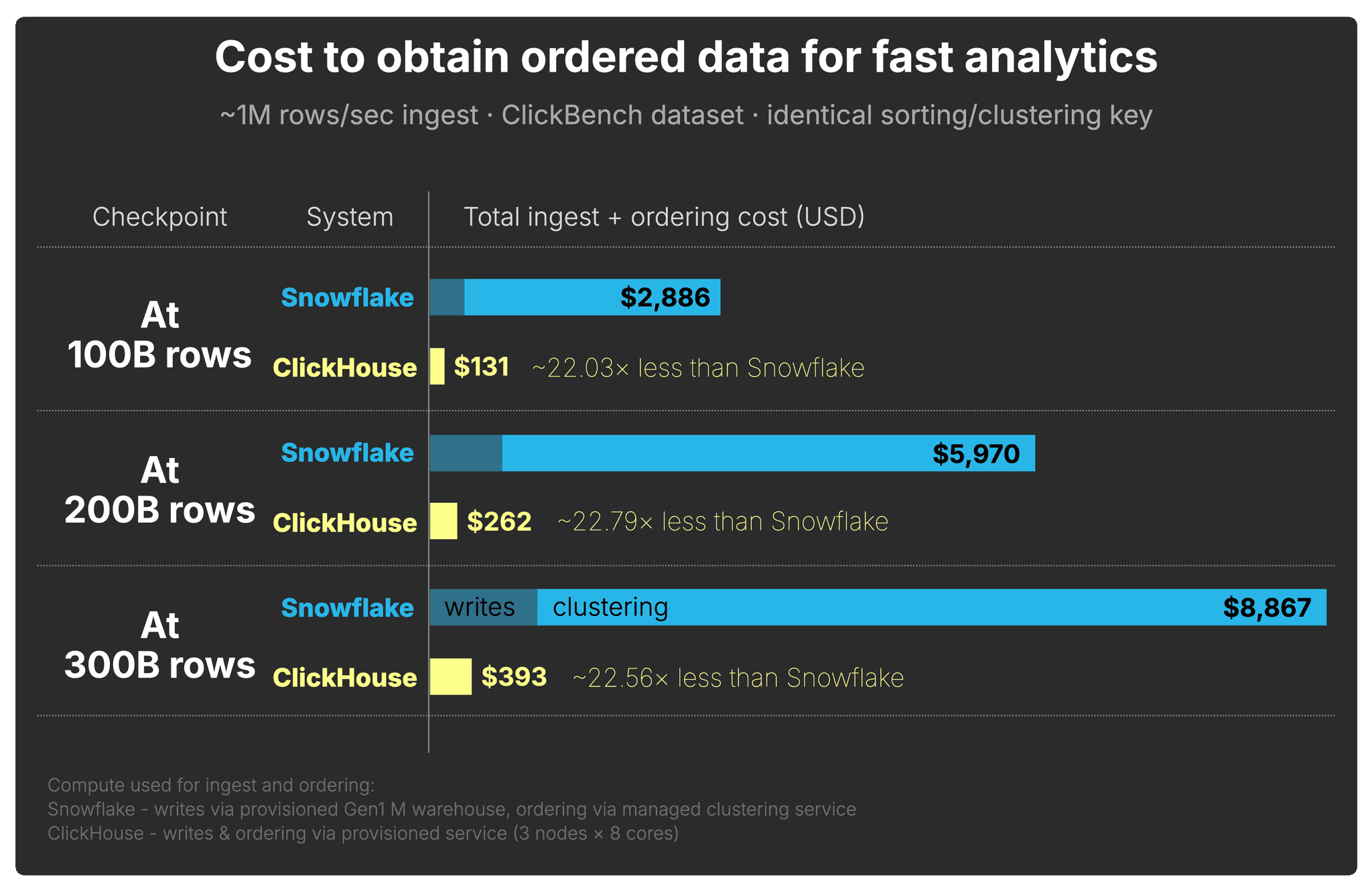
Across all three checkpoints, ClickHouse reaches a query-ready layout at roughly 22× lower cost than Snowflake.
How we measured Snowflake ingest and clustering cost (click to expand)
We split Snowflake’s write-side cost into two parts: the warehouse compute used for ingest and the automatic clustering compute used to obtain ordered data.
For ingest, we used a Gen1 M warehouse. At Enterprise pricing, this warehouse consumes
4 credits per hour. At our sustained ingest rate of roughly 1 million rows per second,
each 100B-row ingest window took roughly 28 hours, so the ingest cost per 100B rows is:
4 credits/hour × $3.00/credit × 28 hours = $336
For clustering, we measured Snowflake’s ordering cost directly from
snowflake.account_usage.automatic_clustering_history, using the
credits_used reported for automatic clustering on the clustered ClickBench table.
The SQL query and its results is available here.
For each 100B-row ingest window, we summed the automatic clustering credits and converted them
using Enterprise pricing at $3 per credit.
The three measured clustering windows used 849.84, 916.09, and
853.59 credits respectively, corresponding to $2,549.52,
$2,748.27, and $2,560.78 of clustering compute.
The total Snowflake ingest + ordering cost shown in the chart is the ingest warehouse cost plus the automatic clustering cost for each 100B-row window.
How we calculated ClickHouse write and ordering cost (click to expand)
For ClickHouse, writes and ordering run on the same provisioned write & ordering service.
In our setup, this service used 3 nodes with 8 CPU cores each.
In ClickHouse Cloud pricing, each 8-core node corresponds to 4 compute units.
Therefore, the 3-node service uses:
3 nodes × 4 compute units/node = 12 compute units
At Enterprise pricing of $0.39 per compute unit per hour, and at our sustained ingest
rate of roughly 1 million rows per second, each 100B-row ingest window took roughly
28 hours. The write and ordering cost per 100B rows is therefore:
12 compute units × $0.39/unit/hour × 28 hours = $131
This includes both ingest and ordering maintenance, because ClickHouse writes sorted data parts and preserves ordering through background merges on the same service.
And as shown earlier, querying that ordered data is also faster and cheaper in ClickHouse.
The write side’s impact on total cost-performance
Where do you get the most query-ready performance per dollar spent on the write side?
To answer that, we combine the total cost to reach the query result with the runtime achieved on that data:
(cost to obtain query-ready data + cost to query that data) × runtime on that data
Smaller is better.
This captures the intuition behind write-side cost-performance:
- Systems with lower cost to obtain query-ready data score better
- Systems with lower query cost score better
- Systems with faster runtimes score better
- Cost and runtime compound; inefficiencies multiply each other
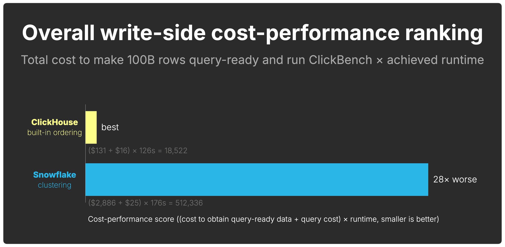
Overall, ClickHouse has a 28× better write-side cost-performance than Snowflake.
What about Interactive Tables, Hybrid Tables, and Dynamic Tables? (click to expand)
Snowflake offers several specialized table types. None of them change the write-side cost analysis for large-scale analytical workloads.
Interactive Tables are designed for low-latency, high-concurrency lookups. The interactive warehouse enforces a hard five-second query timeout on SELECT queries that cannot be increased - by design, to protect the cache from long-running scans. With 43 ClickBench queries completing in a combined 176 seconds on 100B ordered rows, a number of individual queries run well past the five-second cutoff and would be cancelled before returning a result. Interactive Tables are also optimized for simple, selective queries; the docs explicitly advise against large joins, complex aggregations, and high-cardinality clustering keys such as timestamps.
Hybrid Tables use row-based storage, optimized for transactional point lookups rather than analytical range scans. They are capped at 2 TB of row-store data per Snowflake database. In our benchmark, Snowflake stored 3.11 TB at 100B rows - already over the hybrid table quota. Hybrid Tables also do not support clustering keys, Snowpipe Streaming, or materialized views, and queries do not use the result cache.
Dynamic Tables pre-materialize transformed query results on a configurable refresh lag. They are useful for building incremental data pipelines and pre-aggregated views, but they do not change how the underlying event data is stored or ordered. The base table still requires clustering for analytical queries to prune effectively, and each refresh runs on warehouse compute and is billed accordingly. Dynamic Tables address a different problem - they do not reduce the write-side cost of keeping raw data query-ready.
Ordering cost is only one part of write-side cost-performance.
Ordering architecture also changes the storage footprint
The storage layout that results from that ordering also affects how much data is stored, how much has to be read later, and how much I/O future queries perform.
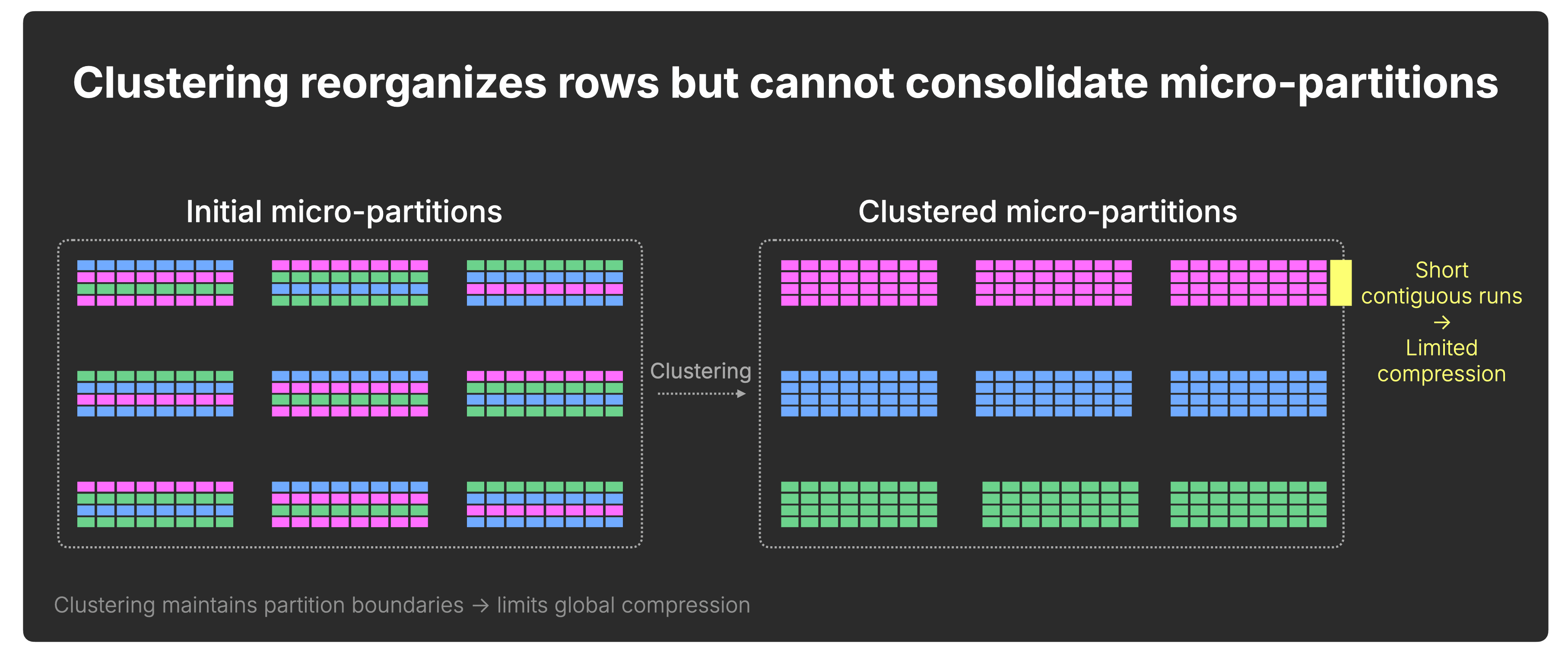
Snowflake: redistribution without consolidation
Snowflake micro-partitions remain bounded in size, typically 50–500 MB before compression.
As a result, clustering redistributes rows across partitions but does not structurally consolidate the dataset.
Contiguous value runs cannot extend beyond micro-partition boundaries, and compression improvements are bounded by partition size:
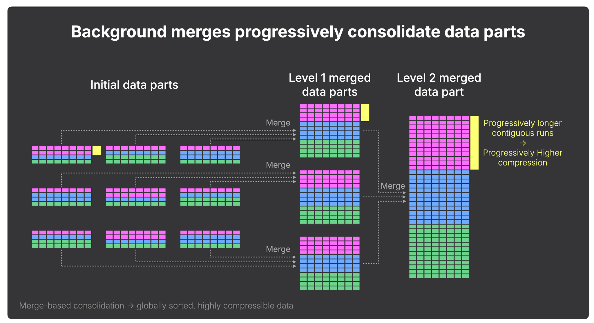
ClickHouse: progressive consolidation over time
In ClickHouse, data is progressively consolidated over time.
Background merges continuously combine smaller parts into larger ones, eventually producing parts of roughly ~150 GB compressed, which can correspond to 1 TB or more of uncompressed data depending on compression ratio.
These merges do more than reorganize rows, they consolidate the dataset.
With each merge, contiguous runs of values grow longer, allowing compression to improve across progressively larger segments of the table:
Importantly, consolidation does not reduce pruning granularity. ClickHouse still prunes at the granule level (typically row blocks with a size of ~10 MB before compression), driven by the sparse primary index, even inside large merged parts.
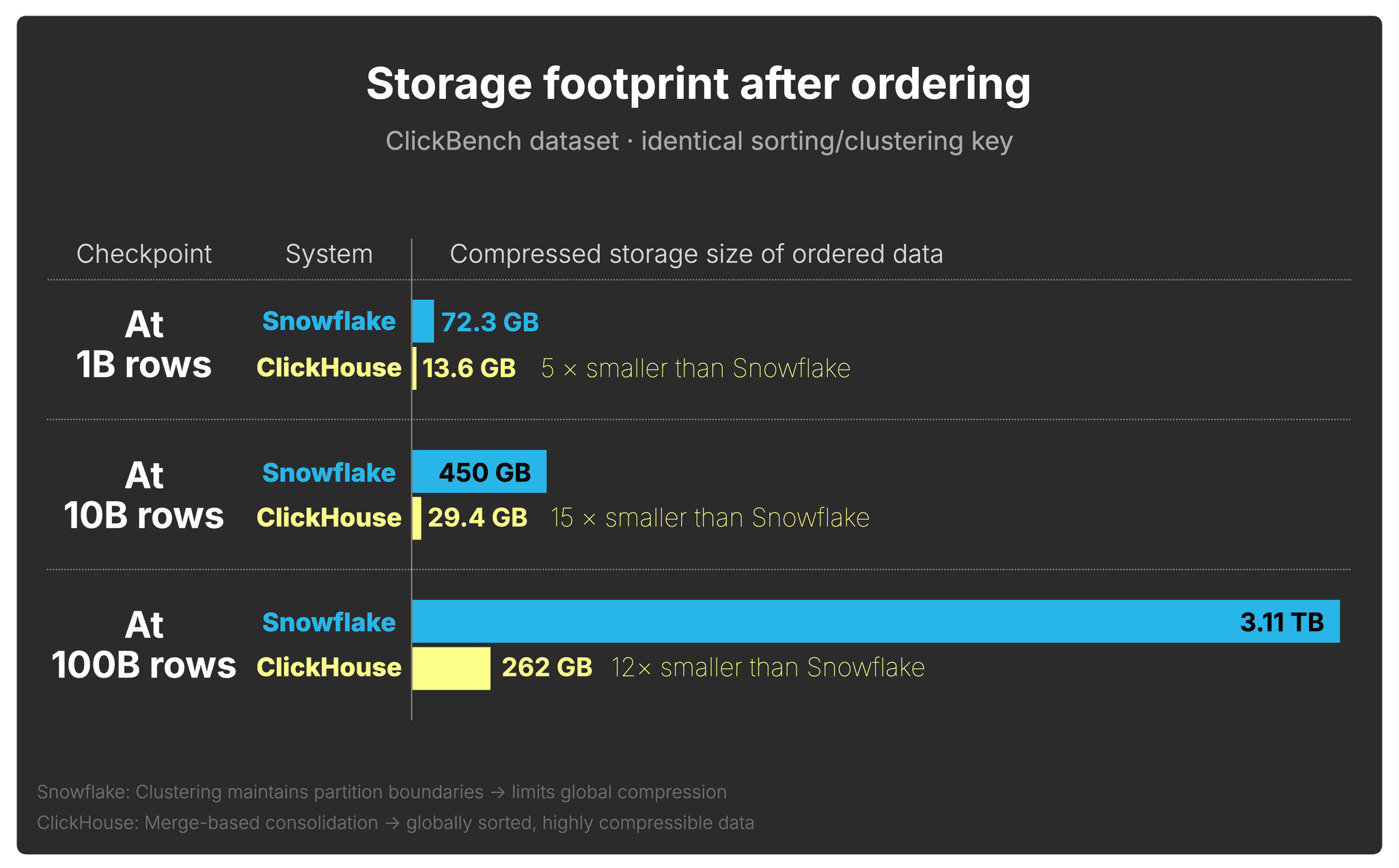
How storage footprint diverges at scale
Under continuous ingest into unbounded tables, this structural difference compounds over time.
Using the same continuously ingested web analytics data from the previous section, clustered and sorted on the identical key in both systems, we now examine how the compressed footprint diverges as the table grows to 1B, 10B, and 100B rows (storage measured via Snowflake TABLE_STORAGE_METRICS and ClickHouse system.parts):
A note on storage vs. compute costs (click to expand)
In many analytical workloads, compute dominates raw storage spend. However, a larger
physical footprint means:
- More data loaded per query
- Lower cache residency
- Higher I/O pressure
- Increased object storage latency exposure
In other words, compression directly influences query execution behavior, not just monthly storage spend.
Even with clustering enabled and identical sorting keys, Snowflake stores 5×–15× more compressed data than ClickHouse on the ClickBench dataset, increasing both storage cost and downstream query I/O.
This concludes our exploration of how the storage layers of two modern cloud data warehouses organize and maintain ingested data over time.
Built for the pressure of agentic analytics
Agentic analytics raises the pressure on every layer of the database.
New data pours in every second and never stops. Users and agents expect fast, complex insights over that data immediately: fraud detection, operational alerts, AI analyst workflows, real-time investigations. The system has to keep up before the query even starts.
That is the write side of cost-performance.
In this benchmark, ClickHouse reached a query-ready layout at roughly 22× lower cost than Snowflake across the 100B, 200B, and 300B row checkpoints. Combined with the faster query runtime achieved on that ordered data, ClickHouse delivered 28× better write-side cost-performance.
The reason is architectural. ClickHouse orders data through its storage layer as it is written, then incrementally refines that layout through background merges. There is no separate clustering service, no separate clustering charge, and no dependency on a background process finishing before queries over fresh data can benefit from pruning.
This matters even more in real deployments. Our test used a single table, a single steady ingest stream, and a modest 1 million rows per second ingest rate. Multiply that by many event streams, higher ingest rates, and many tables, and the cost of keeping data query-ready becomes part of the core economics of the platform.
There is another compounding effect: storage footprint. Because ClickHouse progressively consolidates sorted data, compression improves as the table grows. In our test, Snowflake stored 15× more data than ClickHouse on the same ClickBench dataset, even with clustering enabled on the identical key. That means the write-path difference also shows up later as higher storage cost and more downstream query I/O.
Combined with the order-of-magnitude read-side advantage from our previous study, ClickHouse leads at both ends of the analytics pipeline.
ClickHouse is purpose-built for cost-efficient real-time analytics at massive scale. In the agentic era, that starts with the write path.
Get started with ClickHouse Cloud today and receive $300 in credits. At the end of your 30-day trial, continue with a pay-as-you-go plan, or contact us to learn more about our volume-based discounts. Visit our pricing page for details.