ClickHouse Release 25.9

Another month goes by, which means it’s time for another release!

ClickHouse version 25.9 contains 25 new features 🍎 22 performance optimizations 🍁 83 bug fixes 🌿

This release brings automatic global join reordering, streaming for secondary indices, a new text index, and more!

New contributors #

A special welcome to all the new contributors in 25.9! The growth of ClickHouse's community is humbling, and we are always grateful for the contributions that have made ClickHouse so popular.

Below are the names of the new contributors:

Aly Kafoury, Christian Endres, Dmitry Prokofyev, Kaviraj, Max Justus Spransy, Mikhail Kuzmin, Sergio de Cristofaro, Shruti Jain, c-end, dakang, jskong1124, polako, rajatmohan22, restrry, shruti-jain11, somrat.dutta, travis, yanglongwei

Hint: if you’re curious how we generate this list… here.

You can also view the slides from the presentation.

Join reordering #

Contributed by Vladimir Cherkasov #

A long-standing dream for many ClickHouse users has come true in this release: automatic global join reordering.

ClickHouse can now reorder complex join graphs spanning dozens of tables, across the most common join types (inner, left/right outer, cross, semi, anti). Automatic global join reordering uses the fact that joins between more than two tables are associative.

Why join order matters #

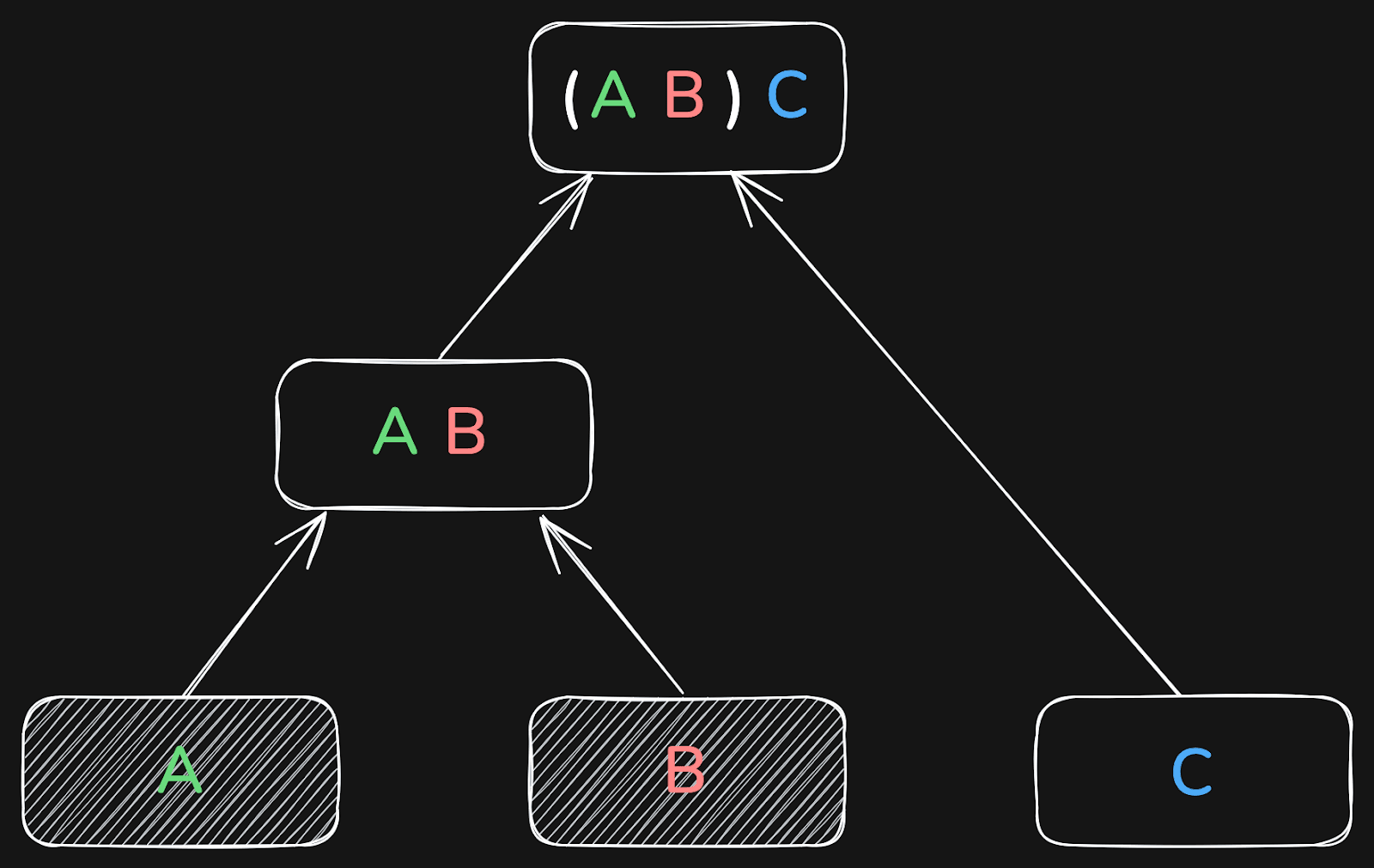
For example, a database may choose to first join tables A and B, and then the result of that with table C:

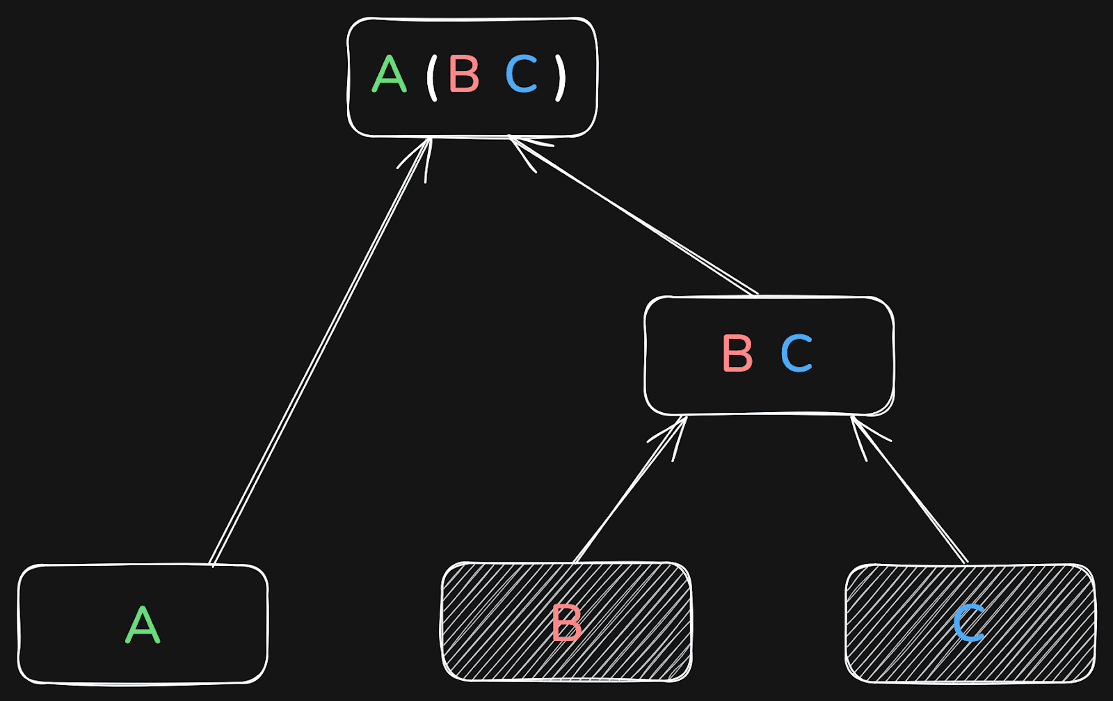
Or it may first join B and C, and the result of that with table A:

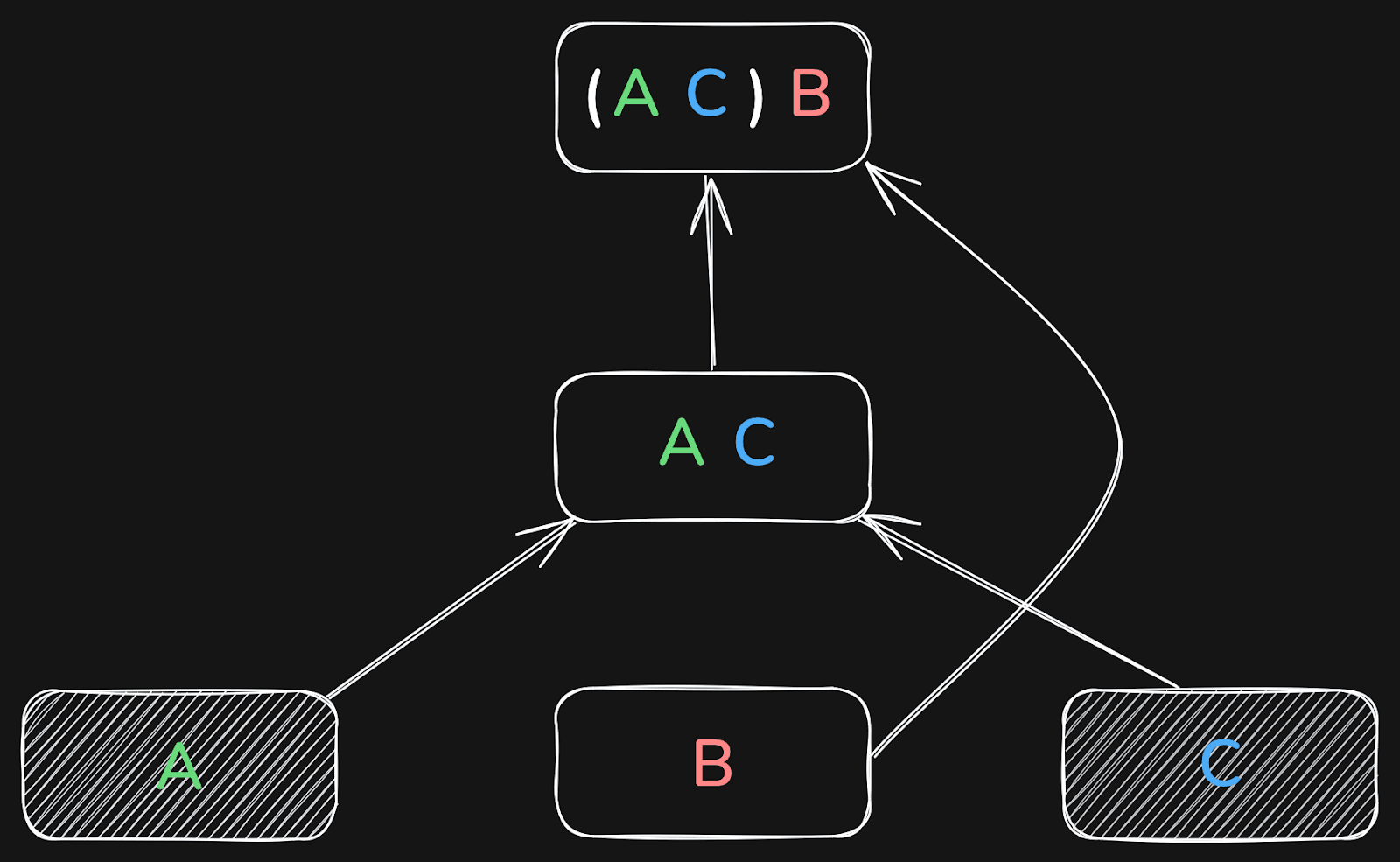
Or it first joins A and C, and the result of that with B:

The result will be the same in all three cases.

The more tables are joined, the more important the global join order becomes.

In some cases, good and bad join orders can differ by many orders of magnitude in runtime!

To see why join order matters so much, let’s briefly recap how ClickHouse executes joins.

How ClickHouse joins work #

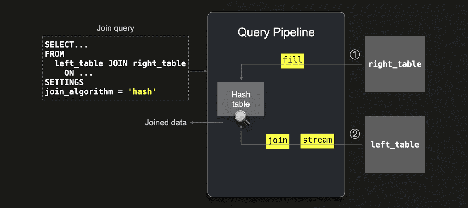
As a brief recap: ClickHouse’s fastest join algorithms, including the default parallel hash join, have two phases:

Build phase: loading the right-hand side table into an in-memory hash table(s).
Probe phase: streaming the left-hand side table and performing lookups into the hash table(s).

Because the build side is loaded into memory upfront, placing the smaller table on the right-hand side of the join is usually far more efficient.

Other join algorithms, such as the partial merge join (which uses external sorting rather than in-memory hash tables), also have build and probe phases. Here, too, placing the smaller table on the build side makes execution faster.

Local join reordering #

Automatic local join reordering for two joined tables was first introduced in 24.12. This optimization moves the small of both tables to the right (build) side and therefore reduces the effort needed to build the hash table.

Global join reordering #

In 25.9, ClickHouse introduced global join reordering to determine the optimal join order (build vs probe) of more than two tables during query optimization.

Global join order optimization is much more challenging than local optimization. As the number of possible join orders grows exponentially with the number of joined tables, ClickHouse cannot explore the search space exhaustively. The database instead runs a greedy optimization algorithm to converge to a “good enough” join order quickly.

The optimization algorithm also requires cardinality estimations of the join columns - i.e. how many rows are two joined tables expected to contain (considering additional WHERE filters on them). The cardinality estimations are provided using row count estimates from the storage engines or column statistics (if available).

As of today, column statistics must be created manually (see our example below). We plan to create column statistics for new tables automatically in future versions of ClickHouse.

Controlling join reordering #

Two new settings control the global join reordering:

query_plan_optimize_join_order_limit - Value is the max number of tables to apply the reordering to.
allow_statistics_optimize - Allows using statistics to optimize join order

Benchmarks: TPC-H results #

Let’s see it in action on the classic TPC-H join benchmark.

To evaluate the impact of global join reordering with column statistics, we created two versions of the TPC-H schema (scale factor 100) on an AWS EC2 m6i.8xlarge instance (32 vCPUs, 128 GiB RAM):

Without statistics: the 8 TPC-H tables created with the default DDL.
With statistics: the same 8 tables extended with column statistics.

Once those tables are created, we can use the commands in this script to load the data.

If you want to follow along, the commands to create and load the tables are included in the links above.


1CREATE DATABASE tpch_no_stats;
2USE tpch_no_stats;
3-- Create the 8 tables with the default DDL
4-- Load data


1CREATE DATABASE tpch_stats;
2USE tpch_stats;
3-- Create the 8 tables with extended DDL (with column statistics)
4-- Load data

We then ran the following TPC-H query, which contains a join across six tables, as our test query:


1SELECT
2  n_name,
3  sum(l_extendedprice * (1 - l_discount)) AS revenue
4FROM
5  customer, 
6  orders, 
7  lineitem, 
8  supplier, 
9  nation, 
10  region
11WHERE
12  c_custkey = o_custkey
13AND l_orderkey = o_orderkey
14AND l_suppkey = s_suppkey
15AND c_nationkey = s_nationkey
16AND s_nationkey = n_nationkey
17AND n_regionkey = r_regionkey
18AND r_name = 'ASIA'
19AND o_orderdate >= DATE '1994-01-01'
20AND o_orderdate < DATE '1994-01-01' + INTERVAL '1' year
21GROUP BY
22  n_name
23ORDER BY
24  revenue DESC;

First, we executed the query on the tables without statistics:


1USE tpch_no_stats;
2SET query_plan_optimize_join_order_limit = 10;
3SET allow_statistics_optimize = 1;
4
5-- test_query

   ┌─n_name────┬─────────revenue─┐
1. │ VIETNAM   │  5310749966.867 │
2. │ INDIA     │ 5296094837.7503 │
3. │ JAPAN     │ 5282184528.8254 │
4. │ CHINA     │ 5270934901.5602 │
5. │ INDONESIA │ 5270340980.4608 │
   └───────────┴─────────────────┘

5 rows in set. Elapsed: 3903.678 sec. Processed 766.04 million rows, 16.03 GB (196.23 thousand rows/s., 4.11 MB/s.)
Peak memory usage: 99.12 GiB.

That took over one hour! 🐌 And used 99 GiB of main memory.

Then we repeated the same query on the tables with statistics:


1USE tpch_stats;
2SET query_plan_optimize_join_order_limit = 10;
3SET allow_statistics_optimize = 1;
4
5-- test_query

Query id: 5c1db564-86d0-46c6-9bbd-e5559ccb0355

   ┌─n_name────┬─────────revenue─┐
1. │ VIETNAM   │  5310749966.867 │
2. │ INDIA     │ 5296094837.7503 │
3. │ JAPAN     │ 5282184528.8254 │
4. │ CHINA     │ 5270934901.5602 │
5. │ INDONESIA │ 5270340980.4608 │
   └───────────┴─────────────────┘

5 rows in set. Elapsed: 2.702 sec. Processed 638.85 million rows, 14.76 GB (236.44 million rows/s., 5.46 GB/s.)
Peak memory usage: 3.94 GiB.

Now it took 2.7 seconds. ~1,450× faster than before. With ~25x less memory usage.

What’s next for join reordering #

This is just the first step for global join reordering in ClickHouse. Today, it requires manually created statistics. The next steps will include:

Automatic statistics creation — removing the need for manual setup.
Support more join types (like outer joins) and joins over subqueries
More powerful join reordering algorithms — handling larger join graphs and more complex scenarios.

Stay tuned.

Streaming for secondary indices #

Contributed by Amos Bird #

Before ClickHouse 25.9, secondary indices (e.g., minmax, set, bloom filter, vector, text) were evaluated before reading the underlying table data.

Before: Sequential index scans #

The index entries are scanned upfront to decide which granules (the smallest processing units in ClickHouse, typically covering 8,192 rows each) may contain matching rows for a query’s WHERE filter.

The following animation illustrates this process:

① Index scan and granule selection - ClickHouse checks each index entry to determine which granules to read. Only matching granules are chosen; the others are skipped.

② Query execution - The selected granules are streamed into the query engine and processed into the final result.

This sequential process has a few drawbacks:

Inefficient with LIMIT: Even if a query stops early due to a LIMIT, ClickHouse still has to scan the entire index upfront (and may select more data than necessary).
Startup delay: Index analysis happens before the actual query execution begins.
Heavy index scans: In some cases (e.g., queries with highly selective WHERE filters over huge tables), scanning the index can cost more than scanning and processing the selected data itself.

Now: Streaming secondary indices #

ClickHouse 25.9 eliminates these drawbacks by interleaving data reads with index checks, as shown in the animation below:

① Index scan, granule selection, and ② query execution (concurrent) – When ClickHouse is about to read a table data granule (e.g. because it was selected by the primary index analysis), it first checks the corresponding secondary index entry (if one exists). If the secondary index indicates the table granule can be skipped, it’s never read. Otherwise, the granule is read and processed by the query engine, while scanning continues on subsequent granules.

This incremental, two-stream process—reading table granules alongside checking their secondary index entries—is why we call the feature streaming secondary indices (controlled by the setting use_skip_indexes_on_data_read) .

(Note: For simplicity, the animation shows a single-threaded query engine, but in reality multiple threads process many granules concurrently.)

This concurrent execution eliminates the startup delay and avoids wasted work. For example, with queries that stop early due to a LIMIT, ClickHouse halts index checks and granule reads as soon as the result is complete.

Demo: Faster results with streaming secondary indices #

In the release webinar, Alexey demonstrated streaming secondary indices on massive ClickHouse tables containing trillions of log records from test runs applied to pull requests and commits. On these datasets, some individual secondary indices alone exceed 6 TB compressed.

Since reproducing that scale isn’t practical, we’ll use a simplified artificial example that you can run yourself.

We ran the experiment on an AWS EC2 m6i.8xlarge instance (32 vCPUs, 128 GiB RAM).

First, we created a table with a String column and added a Bloom filter index on that column:


1CREATE TABLE test (
2  s String, 
3  index s_idx s type bloom_filter(0.0001) granularity 1
4)
5ENGINE = MergeTree
6ORDER BY () 
7SETTINGS index_granularity = 1024;

Next, we inserted one billion rows:


1INSERT INTO test 
2SELECT if(number % 1024 == 0, 'needle', randomPrintableASCII(64)) 
3FROM numbers_mt(1_000_000_000);

We can check that the bloom filter index has a size of over 2 GiB now:


1SELECT 
2  name, 
3  type_full, 
4  formatReadableSize(data_uncompressed_bytes) AS size
5FROM system.data_skipping_indices
6WHERE database = 'default' AND table = 'test';

   ┌─name──┬─type_full────────────┬─size─────┐
1. │ s_idx │ bloom_filter(0.0001) │ 2.21 GiB │
   └───────┴──────────────────────┴──────────┘

To make the comparison fair, we cleared the OS page cache before each of the two test query runs below.


1echo 3 | sudo tee /proc/sys/vm/drop_caches >/dev/null

Without streaming indices (use_skip_indexes_on_data_read = 0), finding a single row with LIMIT 1 took ~10 seconds.

Note that we set max_threads = 1 and disabled the query condition cache to isolate and highlight the effect of secondary index processing.


1SELECT * FROM test WHERE s = 'needle' LIMIT 1 
2SETTINGS 
3  max_threads = 1, 
4  use_query_condition_cache = 0,  use_skip_indexes_on_data_read = 0;

   ┌─s──────┐
1. │ needle │
   └────────┘

1 row in set. Elapsed: 10.173 sec. Processed 29.70 thousand rows, 2.14 MB (2.92 thousand rows/s., 210.00 KB/s.)
Peak memory usage: 8.90 MiB.

With streaming indices (use_skip_indexes_on_data_read = 1), the same query returned in ~2.4 seconds — over 4× faster with less memory used.


1SELECT * FROM test WHERE s = 'needle' LIMIT 1 
2SETTINGS 
3  max_threads = 1, 
4  use_query_condition_cache = 0,  use_skip_indexes_on_data_read = 1;

   ┌─s──────┐
1. │ needle │
   └────────┘

1 row in set. Elapsed: 2.471 sec. Processed 29.70 thousand rows, 2.14 MB (12.02 thousand rows/s., 864.57 KB/s.)
Peak memory usage: 4.48 MiB.

As a reminder, the observed speedup comes from two (① and ②) mechanisms:

Without streaming indices: Before query processing even begins, ClickHouse must fully scan and process the index to identify all matching granules.
With streaming indices:
① ClickHouse concurrently scans the index and processes matching granules in the query engine.
② And as soon as the first matching row (LIMIT 1) is found, it immediately stops scanning further index entries and granules, eliminating wasted work.

A new text index #

Contributed by Anton Popov, Elmi Ahmadov, Jimmy Aguilar Mena #

Since publishing our blog on reworking full-text search in August 2025, we’ve learned even more from extended testing. Some approaches we thought were ‘done’ turned out to be stepping stones toward an even better design. We view this as part of ClickHouse’s DNA: we share early, we test rigorously, and we continue to improve until we’re confident that we’ve delivered the fastest solution possible.

The previous FST-based implementation optimized space but was inefficient because it required loading large chunks of data into memory and wasn’t structured around skip index granules, making query analysis more difficult.

The new design makes ClickHouse's text index streaming-friendly and structures data around skip index granules for more efficient queries. In ClickHouse 25.9, we're shipping this new experimental text index to provide more efficient and reliable full-text search.

To enable the text index, we need to set the following:


1SET allow_experimental_full_text_index;

We’ll use the Hacker News example dataset to explore this feature. We can download the CSV file like this:


1wget https://datasets-documentation.s3.eu-west-3.amazonaws.com/hackernews/hacknernews.csv.gz

Next, let’s create a table with a text index on the text column:


1CREATE TABLE hackernews
2(
3    `id` Int64,
4    `deleted` Int64,
5    `type` String,
6    `by` String,
7    `time` DateTime64(9),
8    `text` String,
9    `dead` Int64,
10    `parent` Int64,
11    `poll` Int64,
12    `kids` Array(Int64),
13    `url` String,
14    `score` Int64,
15    `title` String,
16    `parts` Array(Int64),
17    `descendants` Int64,
18    INDEX inv_idx(text)
19    TYPE text(tokenizer = 'default')
20    GRANULARITY 128
21)
22ENGINE = MergeTree
23ORDER BY time;

Now, we can ingest the data:


1INSERT INTO hackernews 
2SELECT *
3FROM file('hacknernews.csv.gz', CSVWithNames);

Let’s check how many records the table contains:


1SELECT count()
2FROM hackernews;

┌──count()─┐
│ 28737557 │ -- 28.74 million
└──────────┘

We’ve got just under 30 million records to work with.

Now let’s see how to query the text column. The hasToken function will use a text index if one exists. searchAll and searchAny will only work if the field has a text index.

To find the users who post the most about OpenAI, we could write the following query:


1select by, count()
2FROM hackernews
3WHERE hasToken(text, 'OpenAI')
4GROUP BY ALL
5ORDER BY count() DESC
6LIMIT 10;

┌─by──────────────┬─count()─┐
│ minimaxir       │      48 │
│ sillysaurusx    │      43 │
│ gdb             │      40 │
│ thejash         │      24 │
│ YeGoblynQueenne │      23 │
│ nl              │      20 │
│ Voloskaya       │      19 │
│ p1esk           │      18 │
│ rvz             │      17 │
│ visarga         │      16 │
└─────────────────┴─────────┘

10 rows in set. Elapsed: 0.026 sec.

If we run that same query on a table without a text index, it takes about 10x longer:

10 rows in set. Elapsed: 1.545 sec. Processed 27.81 million rows, 9.47 GB (17.99 million rows/s., 6.13 GB/s.)
Peak memory usage: 172.15 MiB.

We could also write the following query to find the users who posted the most messages that include both OpenAI and Google:


1select by, count()
2FROM hackernews
3WHERE searchAll(text, ['OpenAI', 'Google'])
4GROUP BY ALL
5ORDER BY count() DESC
6LIMIT 10;

┌─by──────────────┬─count()─┐
│ thejash         │      17 │
│ boulos          │       8 │
│ p1esk           │       6 │
│ sillysaurusx    │       5 │
│ colah3          │       5 │
│ nl              │       5 │
│ rvz             │       4 │
│ Voloskaya       │       4 │
│ visarga         │       4 │
│ YeGoblynQueenne │       4 │
└─────────────────┴─────────┘

10 rows in set. Elapsed: 0.012 sec.

Data lake improvements #

Contributed by Konstantin Vedernikov, Smita Kulkarni #

ClickHouse 25.9 sees further support for data lakes, including:

Support for the ALTER UPDATE and DROP TABLE clauses for Apache Iceberg
A new iceberg_metadata_log system table
ORC and Avro for Apache Iceberg data files
Unity catalog on Azure
Distributed INSERT SELECT for data lakes

arrayExcept #

Contributed by Joanna Hulboj #

ClickHouse 25.9 introduces the arrayExcept function, which enables you to determine the difference between two arrays. An example is shown below:


1SELECT arrayExcept([1, 2, 3, 4], [1, 3, 5]) AS res;

┌─res───┐
│ [2,4] │
└───────┘

Boolean settings #

Contributed by Thraeka #

ClickHouse 25.9 also allows you to define boolean settings without specifying an argument. This means that we can make DESCRIBE output compact, like this:


1SET describe_compact_output;

And no longer need to explicitly specify that it’s true, as we did before 25.9:


1SET describe_compact_output = true;

To disable a setting, we still need to provide the argument as false.

Storage Class specification for S3 #

Contributed by Alexander Sapin #

ClickHouse 25.9 allows you to specify the AWS S3 storage class when using the S3 table engine or table function.

For example, we could use intelligent tiering if we want AWS to optimize storage costs by automatically moving data to the most cost-effective access tier.


1CREATE TABLE test (s String)
2ENGINE = S3('s3://mybucket/test.parquet',
3            storage_class_name = 'INTELLIGENT_TIERING');
4
5INSERT INTO test VALUES ('Hello');


1INSERT INTO FUNCTION s3('s3://mybucket/test.parquet',
2            storage_class_name = 'INTELLIGENT_TIERING') 
3VALUES('test');