ClickHouse Release 25.7

Another month goes by, which means it’s time for another release!

ClickHouse version 25.6 contains 27 new features 🌺 26 performance optimizations 🍦 98 bug fixes 🐞

This release brings

New Contributors #

A special welcome to all the new contributors in 25.7! The growth of ClickHouse's community is humbling, and we are always grateful for the contributions that have made ClickHouse so popular.

Below are the names of the new contributors:

Alon Tal, Andrey Volkov, Damian Maslanka, Diskein, Dominic Tran, Fgrtue, H0uston, HumanUser, Ilya fanyShu, Joshie, Mishmish Dev, Mithun P, Oleg Doronin, Paul Lamb, Rafael Roquetto, Ronald Wind, Shiv, Shivji Kumar Jha, Surya Kant Ranjan, Ville Ojamo, Vlad Buyval, Xander Garbett, Yanghong Zhong, ddavid, e-mhui, f2quantum, jemmix, kirillgarbar, lan, wh201906, xander, yahoNanJing, yangjiang, yangzhong, 思维

Hint: if you’re curious how we generate this list… here.

You can also view the slides from the presentation.

Lightweight updates #

Contributed by Anton Popov #

ClickHouse now supports standard SQL UPDATE statements at scale, powered by a new lightweight patch-part mechanism. Unlike classic mutations, which rewrite full columns, these updates write only tiny “patch parts” that slide in instantly with minimal impact on query performance.

How it works #

Patch parts extend the same principles behind purpose-built engines like ReplacingMergeTree, but in a fully general way, exposed through standard SQL:

UPDATE orders
SET discount = 0.2
WHERE quantity >= 40;

• Inserts are fast.
• Merges are continuous.
• Parts are immutable and sorted.

So instead of locating and modifying rows, ClickHouse simply inserts a compact patch part named for what it does: it patches data parts during merges, applying only the changed data:

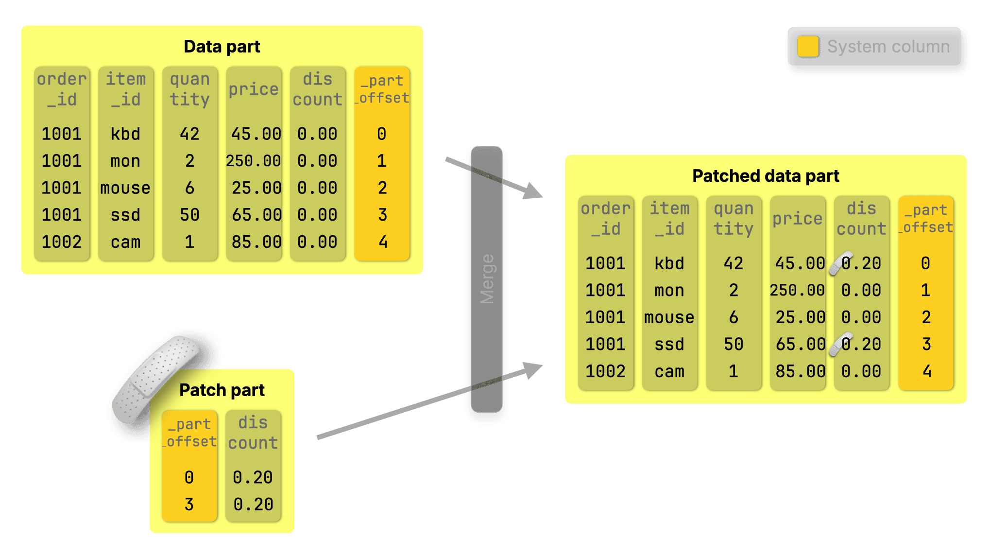
Merges were already running in the background, so we made them do more, with near-zero overhead. They now apply patch parts, updating the base data efficiently as parts are merged.

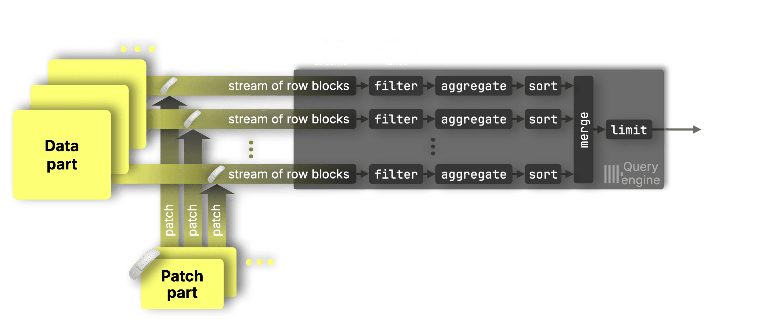
Updates show up right away, not-yet-merged patch parts are matched and applied independently for each data range in each data stream in a surgical, targeted way, ensuring that updates are applied correctly without disrupting parallelism:

This makes declarative updates up to 1,000× faster than before in our benchmarks, with minimal impact on queries before merges.

Whether you’re updating one row or a million, it’s now fast, efficient, and fully declarative.

DELETE are lightweight featherweight #

For DELETES with standard SQL syntax like:

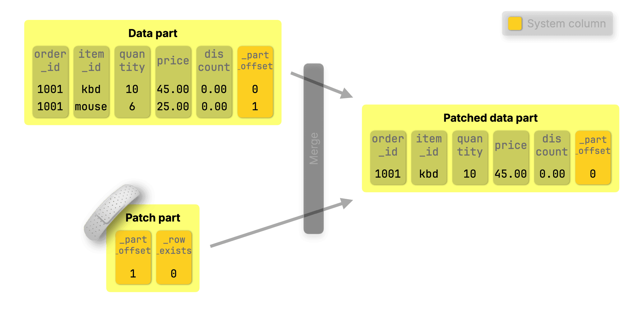
DELETE FROM orders WHERE order_id = 1001 AND item_id = 'mouse';

ClickHouse simply creates a patch part that sets _row_exists = 0 for the deleted rows. The row is then dropped during the next background merge:

Under the hood of fast UPDATEs #

Want to go deeper? Check out our 3-part blog series on fast UPDATEs in ClickHouse:

• Part 1: Purpose-built engines
  Learn how ClickHouse sidesteps slow row-level updates using insert-based engines like ReplacingMergeTree, CollapsingMergeTree, and CoalescingMergeTree.

• Part 2: Declarative SQL-style UPDATEs
  Explore how we brought standard UPDATE syntax to ClickHouse with minimal overhead using patch parts.

• Part 3: Benchmarks
  See how fast it really is. We benchmarked every approach, including declarative UPDATEs, and got up to 1,000× speedups.

• Bonus: ClickHouse vs PostgreSQL
  We put ClickHouse’s new SQL UPDATEs head-to-head with PostgreSQL on identical hardware and data—parity on point updates, up to 4,000× faster on bulk changes.

AI-powered SQL generation #

Contributed by Kaushik Iska #

The ClickHouse client and clickhouse-local now support AI-powered SQL generation. You can enable this by using the ?? prefix, and if you have OPENAI_API_KEY or ANTHROPIC_API_KEY on your path, it will ask if you want to use it.

For example, let’s connect to the ClickHouse SQL Playground:

1./clickhouse client -mn 
2--host sql-clickhouse.clickhouse.com 
3--secure 
4--user demo --password ''

And then we’ll ask for the most popular repositories in July 2025:

1?? what was the most popular github repository in July 2025?;

It will then confirm that we’d like to use our API key:

AI SQL generation will use openai API key from environment variable.
Do you want to continue? [y/N] y

And then off it goes, printing out its thoughts along the way:

• Starting AI SQL generation with schema discovery...
─────────────────────────────────────────────────
🧠 thinking..[INFO] Text generation successful - model: gpt-4o, response_id: chatcmpl-BxBDkKy9sNi1Bw8E26UC8RXNBMrPT
🔧 Calling: list_databases [call_IXv...]
✓ list_databases completed
  └─ Found 37 databases: - amazon - bluesky - country - covid - default - dns - en...
🔧 Calling: list_databases [call_IXv...]
🧠 thinking...✓ list_databases completed
  └─ Found 37 databases: - amazon - bluesky - country - covid - default - dns - en...
🧠 thinking..[INFO] Text generation successful - model: gpt-4o, response_id: chatcmpl-BxBDmOwzsHgBNHtOiT8tEIhjJoMXV
🔧 Calling: list_tables_in_database [call_pRq...]
  └─ Args: {"database":"github"}
🧠 thinking...✓ list_tables_in_database completed
  └─ Found 19 tables in database 'github': - actors_per_repo - actors_per_repo_mv ...
🔧 Calling: list_tables_in_database [call_pRq...]
  └─ Args: {"database":"github"}
✓ list_tables_in_database completed
  └─ Found 19 tables in database 'github': - actors_per_repo - actors_per_repo_mv ...
🧠 thinking...[INFO] Text generation successful - model: gpt-4o, response_id: chatcmpl-BxBDo0qbEkfvzTl6vgrA49fgjVVfo
🔧 Calling: get_schema_for_table [call_NKK...]
  └─ Args: {"database":"github","table":"repo_events_per_day"}
🧠 thinking✓ get_schema_for_table completed
  └─ Schema for github.repo_events_per_day: CREATE TABLE github.repo_events_per_da...
🔧 Calling: get_schema_for_table [call_NKK...]
  └─ Args: {"database":"github","table":"repo_events_per_day"}
✓ get_schema_for_table completed
  └─ Schema for github.repo_events_per_day: CREATE TABLE github.repo_events_per_da...
🧠 thinking.[INFO] Text generation successful - model: gpt-4o, response_id: chatcmpl-BxBDpMp0HpRmFZK2VBZG5y6sWMCsF
─────────────────────────────────────────────────
• ✨ SQL query generated successfully!

Below is the query it came up with:

1SELECT
2    repo_name,
3    sum(count) AS total_events
4FROM github.repo_events_per_day
5WHERE (created_at >= '2025-07-01') AND (created_at <= '2025-07-31')
6GROUP BY repo_name
7ORDER BY total_events DESC
8LIMIT 1;

┌─repo_name───────────────────┬─total_events─┐
│ freefastconnect/fastconnect │       333215 │
└─────────────────────────────┴──────────────┘

I would have also filtered it by event type to only include WatchEvent, but it’s not a bad start. Give it a try and let us know how you get on!

Speed-up for simple aggregations #

Contributed by Amos Bird #

This release brings a targeted optimization for count() aggregations that reduces memory and CPU usage, making these queries even faster.

Parallel aggregation in ClickHouse #

ClickHouse already runs these queries in a highly parallel way, using all available CPU cores, splitting the work across processing lanes, and pushing the hardware close to its limits.

Here’s how it normally works:

① Data streaming
Data is streamed into the engine block by block.

② Parallel processing
Each CPU core processes a disjoint data range: filtering, aggregating, and sorting rows independently.

③ Partial results merge into the ④ final result
Each lane produces partial aggregation states (e.g., a sum and a count for avg()).
These intermediate states are merged into a single final result

Let’s now focus on just one stage of this pipeline: aggregation. This is where each CPU core accumulates partial results, like sums and counts, for its slice of the data, which are later merged into the final answer.

Why partial states are needed #

Partial aggregation states are what make this highly parallel processing model possible, they allow each CPU core to work independently while still contributing to a correct final result.

To understand why partial states are used, consider this query calculating average property prices per town:

SELECT
    town,
    avg(price) AS avg_price
FROM uk_price_paid
GROUP BY town;

Suppose we want the average price in London using two CPU cores:

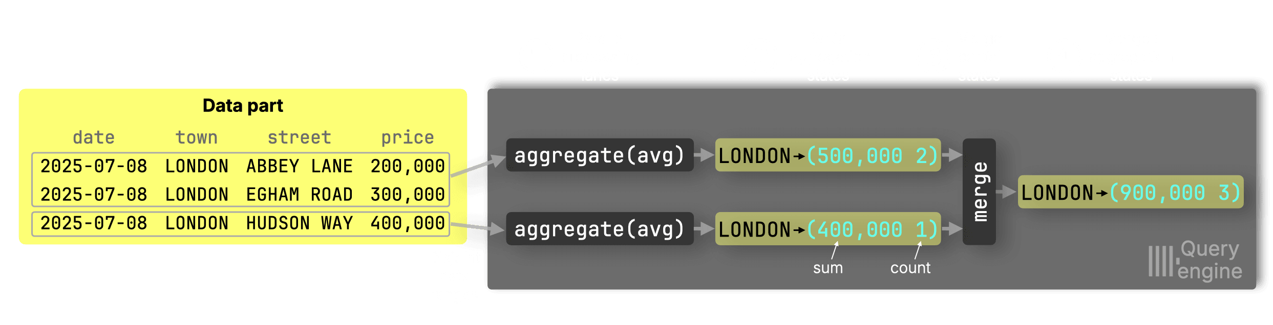
① Parallel processing and ② partial aggregation states

Lane 1 sees two London rows → sum = 500,000, count = 2

Lane 2 sees one London row → sum = 400,000, count = 1

③ Merge into the ④ final state

Final avg = (500,000 + 400,000) / (2 + 1) = 300,000

You must merge sums and counts, not intermediate averages, to avoid errors like:

(250,000 + 400,000) / 2 = 325,000 ← incorrect

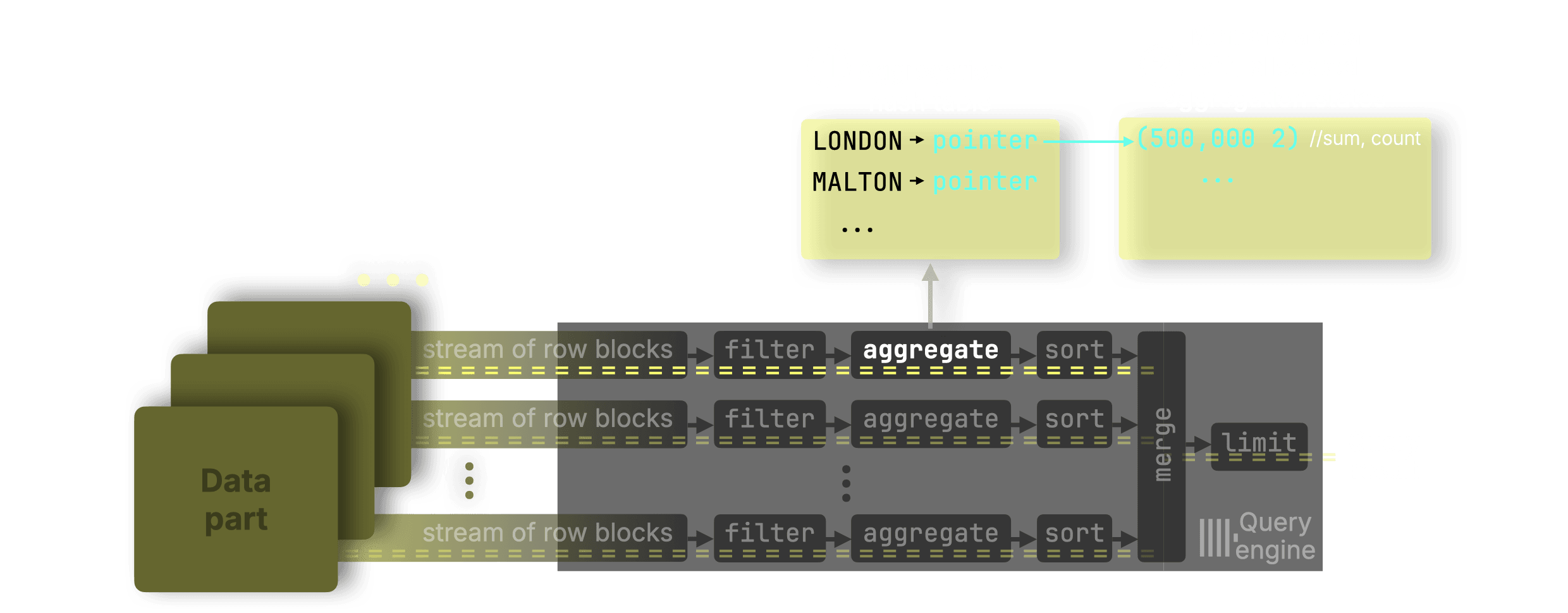
How GROUP BY aggregation works under the hood #

Now let’s zoom in even further, into the internals of the aggregation stage. We’ll see how each processing lane maintains its own hash table and builds aggregation states independently.

GROUP BY queries are processed independently by each lane using a hash aggregation algorithm: each lane maintains a hash table where each key (e.g. town) points to an aggregation state.

For our example, when a processing lane sees LONDON in the input:

• If the key doesn’t exist in the ① hash table, a new entry is created and an aggregation state is allocated in a ② global memory arena. A pointer to that state is stored in the hash table.

• If it does exist, the pointer is used to look up and update the existing aggregation state in the arena.

Optimization for count() #

Now, here’s where this release improves things.

For this query:

SELECT
    town,
    count() AS count
FROM uk_price_paid
GROUP BY town;

…ClickHouse skips the memory arena entirely.

Since count() is an additive function, it doesn’t require a complex aggregation state to correctly merge partial results across lanes. Count() only needs to store a single 64-bit integer (the count itself), which is no larger than a pointer on 64-bit systems, ClickHouse can:

• Store the count directly in the hash table cell
• Skip allocating space in the memory arena
• Skip pointer indirection

This avoids memory allocation and pointer chasing altogether, reducing CPU and memory overhead.

In our tests, count() aggregations are now 20–30% faster than before, with lower memory usage and fewer CPU cycles.

Why this matters #

Count aggregations are everywhere: from dashboards ranking the most active users or most downloaded packages, to alerting systems tracking unusual event frequencies. Whether it’s analytics, observability, or search, nearly every system relies on fast, efficient count queries. That’s why even small improvements here can have an outsized impact.

Real-world results #

We’ll demonstrate this optimization using a typical analytical query over web analytics data that returns the 10 most active users by using a count() aggregation:

SELECT UserID, count() 
FROM hits 
GROUP BY UserID 
ORDER BY count() DESC 
LIMIT 10;

(You can run the query yourself by creating the table and loading the data)

We used an AWS m6i.8xlarge EC2 instance (32 cores, 128 GB RAM) with a gp3 EBS volume (16k IOPS, 1000 MiB/s max throughput) to run the query.

We ran the query 3 times on ClickHouse 25.6, and show the runtime statistics returned by clickhouse-client:

10 rows in set. Elapsed: 0.447 sec. Processed 100.00 million rows, 799.98 MB (223.49 million rows/s., 1.79 GB/s.)
Peak memory usage: 2.50 GiB.

10 rows in set. Elapsed: 0.391 sec. Processed 100.00 million rows, 799.98 MB (255.79 million rows/s., 2.05 GB/s.)
Peak memory usage: 2.52 GiB.

10 rows in set. Elapsed: 0.383 sec. Processed 100.00 million rows, 799.98 MB (261.21 million rows/s., 2.09 GB/s.)
Peak memory usage: 2.51 GiB.

We then ran the same query 3 times on ClickHouse 25.7:

10 rows in set. Elapsed: 0.305 sec. Processed 100.00 million rows, 799.98 MB (327.54 million rows/s., 2.62 GB/s.)
Peak memory usage: 2.00 GiB.

10 rows in set. Elapsed: 0.265 sec. Processed 100.00 million rows, 799.98 MB (377.43 million rows/s., 3.02 GB/s.)
Peak memory usage: 1.96 GiB.

10 rows in set. Elapsed: 0.237 sec. Processed 100.00 million rows, 799.98 MB (422.34 million rows/s., 3.38 GB/s.)
Peak memory usage: 1.96 GiB.

Let's analyse these runs:

ClickHouse 24.06 #

Run	Time (s)	Rows/s (M)	GB/s	Memory (GiB)
1	0.447	223.49	1.79	2.50
2	0.391	255.79	2.05	2.52
3	0.383	261.21	2.09	2.51

Averages:

• Time: 0.407 s

• Rows/s: 246.83 M

• GB/s: 1.98 GB/s

• Memory: 2.51 GiB

ClickHouse 24.07 #

Run	Time (s)	Rows/s (M)	GB/s	Memory (GiB)
1	0.305	327.54	2.62	2.00
2	0.265	377.43	3.02	1.96
3	0.237	422.34	3.38	1.96

Averages:

• Time: 0.269 s

• Rows/s: 375.77 M

• GB/s: 3.01 GB/s

• Memory: 1.97 GiB

Improvements from 24.06 → 24.07 #

Metric	24.06 Avg	24.07 Avg	Improvement
Query time	0.407 s	0.269 s	1.51× faster (34% faster)
Rows/s	246.83 M	375.77 M	1.52× higher
GB/s	1.98 GB/s	3.01 GB/s	1.52× higher
Memory usage	2.51 GiB	1.97 GiB	21.5% less memory

Optimizations for JOINs #

Contributed by Nikita Taranov. #

Over the past few months, improving JOIN performance has been a continuous focus for us. The default JOIN strategy, the parallel hash join, has seen steady optimizations:

• Version 24.7 improved hash table allocation.

• Version 24.12 added automatic join reordering to intelligently choose the optimal table for the build phase.

• versions 25.1 and 25.2 delivered further low-level enhancements, speeding up the join’s probe phase and eliminating thread contention in its build phase, respectively.

These ongoing improvements in parallelism, query planning, and algorithm efficiency have steadily boosted JOIN speeds. ClickHouse 25.7 continues this trend with four additional low-level optimizations for hash joins:

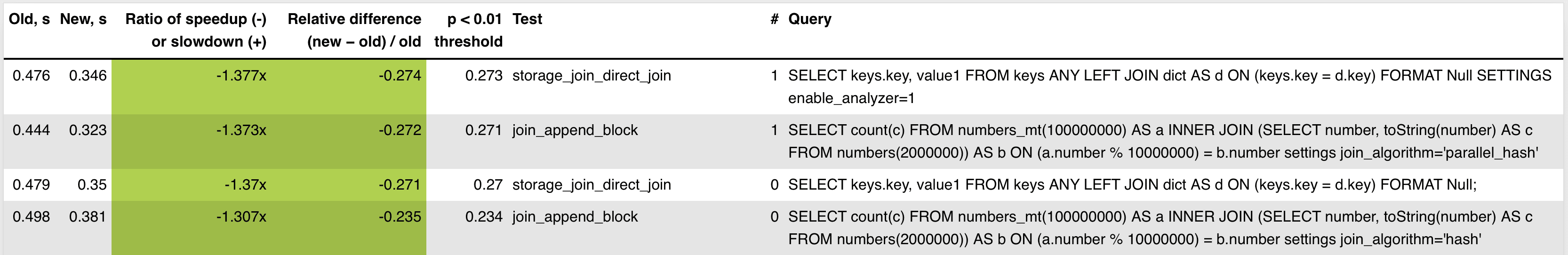
1. Faster single-key joins #

Eliminated an internal loop and unnecessary null-checks for joins on a single key column. This reduces CPU instructions and speeds up one-column JOINs.

Each bar in the PR’s test screenshot compares old vs. new JOIN performance, showing ~1.37× speedups across the board.

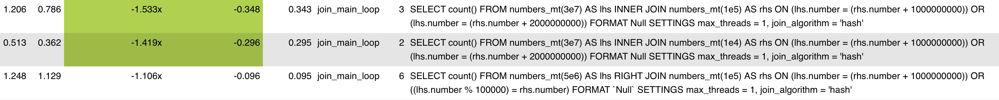
2. Speed-ups for multi-OR-condition JOINs #

Extended those single-key optimizations to JOINs with multiple OR conditions in the ON clause. These now benefit from the same lower-level improvements, making JOINs with multiple OR conditions more efficient.

Multi-condition JOINs now run up to 1.5× faster. Each bar in the PR’s performance test screenshot shows speedups for queries with OR conditions in the ON clause, thanks to reduced instruction overhead and tighter join loop execution.

3. Lower CPU overhead in join processing #

Removed repeated hash computations during join tracking, cutting down on redundant work and boosting JOIN throughput.

Two join queries with large input tables show 1.5× to 1.8× speedups in the PR’s performance test screenshot after reducing hash recomputation overhead. These improvements target joins with high match cardinality, where redundant hashing previously dominated CPU cycles.

4. Reduced memory usage for join results #

Result buffers are now sized precisely after determining the number of matches, avoiding waste and improving performance, especially for wide rows with repeated or padded columns, such as from JOIN ... USING queries or synthetic columns.

The PR’s performance test screenshot shows that JOINs with wide result rows now complete 1.3× to 1.4× faster due to more precise sizing of result buffers. These queries previously over-allocated memory for joined rows, especially when many columns were repeated or padded. The optimization reduces memory usage and speeds up processing for sparse or wide joins.

We’re not done yet. JOIN performance remains a top priority, and we’ll continue optimizing the parallel hash join and other strategies in future releases.

Coming soon: We’re working on a technical deep dive that will walk through all of the JOIN improvements from the past few months, including benchmarks and practical examples. Stay tuned!

Native support for Geo Parquet types #

Contributed by Konstantin Vedernikov #

In ClickHouse 25.5, ClickHouse added support for reading Geo types in Parquet files. In that release, ClickHouse read Parquet’s Geo Types into other ClickHouse types, like tuples or lists.

As of 25.7, ClickHouse reads all Geo types with WKB encoding) into the equivalent ClickHouse Geo type.

Let’s have a look at how it works. The following query writes each of the ClickHouse Geo types into a Parquet file:

1SELECT (10, 10)::Point as point,
2  [(0, 0), (10, 0), (10, 10), (0, 10)]::LineString AS lineString,
3  [
4    [(0, 0), (10, 0), (10, 10), (0, 10)], 
5    [(1, 1), (2, 2)]
6  ]::MultiLineString AS multiLineString,
7  [[(20, 20), (50, 20), (20, 50)], [(30, 30), (50, 50), (50, 30)]]::Polygon AS polygon,
8  [ [[(0, 0), (10, 0), (10, 10), (0, 10)]],
9    [[(20, 20), (50, 20), (50, 50), (20, 50)],[(30, 30), (50, 50), (50, 30)]]
10  ]::MultiPolygon AS multiPolygon,
11  [(0, 0), (10, 0), (10, 10), (0, 10)]::Ring AS ring
12INTO OUTFILE 'geo.parquet' TRUNCATE;

We can then read the Parquet file back:

1DESCRIBE file('geo.parquet');

┌─name────────────┬─type────────────────────────┐
│ point           │ Point                       │
│ lineString      │ LineString                  │
│ multiLineString │ MultiLineString             │
│ polygon         │ Polygon                     │
│ multiPolygon    │ MultiPolygon                │
│ ring            │ Array(Tuple(               ↴│
│                 │↳    `1` Nullable(Float64), ↴│
│                 │↳    `2` Nullable(Float64))) │
└─────────────────┴─────────────────────────────┘

All the types have been read back as their Geo type, except for Ring. Geo types in Parquet typically use WKB encoding, but this doesn't support the Ring type.

New Geospatial functions #

Contributed by Paul Lamb #

Two new functions check whether two polygons intersect: polygonIntersectsCartesian and polygonIntersectsSpherical. polygonIntersectsCartesian uses Cartesian (flat plane) geometry to do the calculation, whereas polygonIntersectsSpherical uses spherical geometry.

Let’s have a look at how to use polygonIntersectsSpherical with the help of two polygons covering parts of central London:

1select polygonsIntersectSpherical(
2  [[[(-0.140, 51.500), (-0.140, 51.510), (-0.120, 51.510), (-0.120, 51.500), (-0.140, 51.500)]]],
3  [[[(-0.135, 51.505), (-0.135, 51.515), (-0.115, 51.515), (-0.115, 51.505), (-0.135, 51.505)]]]
4);

┌─polygonsInte⋯51.505)]]])─┐
│                        1 │
└──────────────────────────┘

And now polygonIntersectsCartesian with imaginary coordinates of two football/soccer players playing on opposite sides of the pitch.

1select polygonsIntersectCartesian(
2[[[(0.0, 0.0), (0.0, 64.0), (45.0, 64.0), (45.0, 0.0), (0.0, 0.0)]]],
3[[[(55.0, 0.0), (55.0, 64.0), (100.0, 64.0), (100.0, 0.0), (55.0, 0.0)]]]
4);

┌─polygonsInte⋯51.505)]]])─┐
│                        1 │
└──────────────────────────┘

Security features #

Contributed by Artem Brustovetskii / Diskein #

This release had a couple of security features.

First, you can now create users dynamically using parameterized queries, making user provisioning more flexible:

1SET param_username = 'test123';
2CREATE USER {username:Identifier};

This feature allows for programmatic user creation with variable usernames, improving automation capabilities for user management workflows.

And we can now configure READ and WRITE grants for external data sources. Previously, external data access was managed with broad permissions:

1GRANT S3 ON *.* TO user

In 25.7, you can enable the new read/write grants feature in your configuration:

1# config.d/read_write_grants.yaml
2access_control_improvements:
3  enable_read_write_grants: true

And then grant permissions like this:

1GRANT READ, WRITE ON S3 TO user;