ClickHouse vs. Elasticsearch: The Mechanics of Count Aggregations

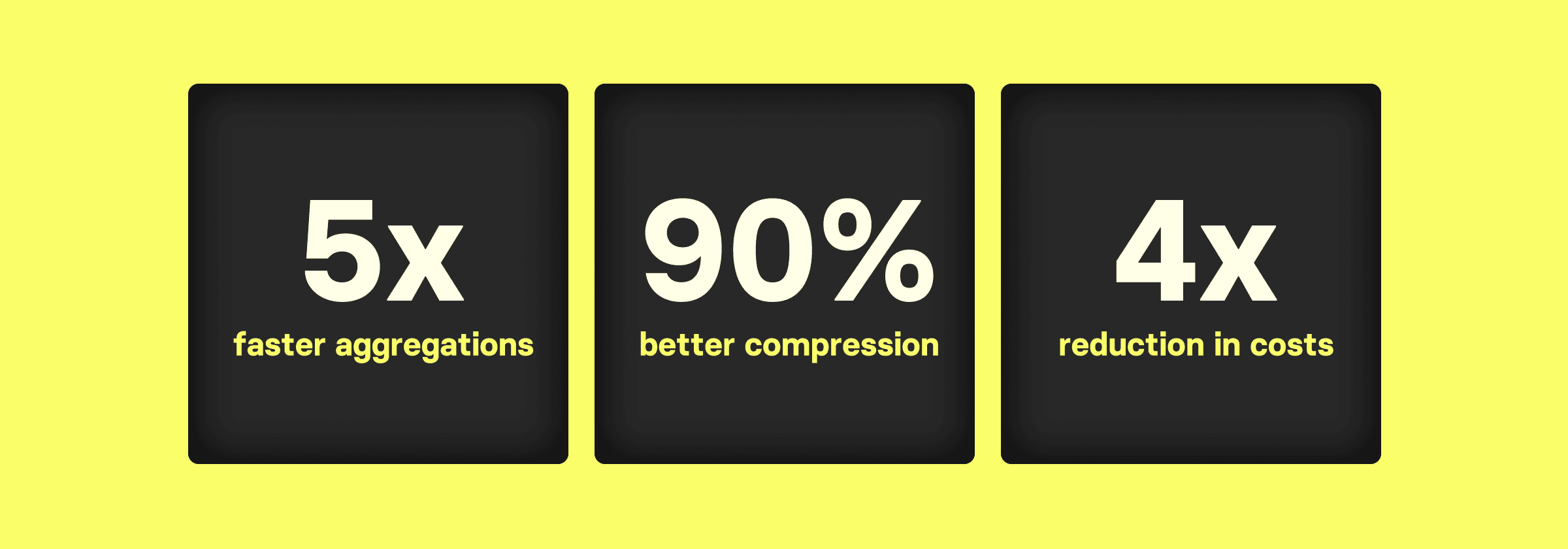
In another blog post, we examined the performance of ClickHouse vs. Elasticsearch on a workload commonly present in large-scale data analytics and observability use cases – count(*) aggregations over billions of table rows. We showed that ClickHouse vastly outperforms Elasticsearch for running aggregation queries over large data volumes. Specifically:

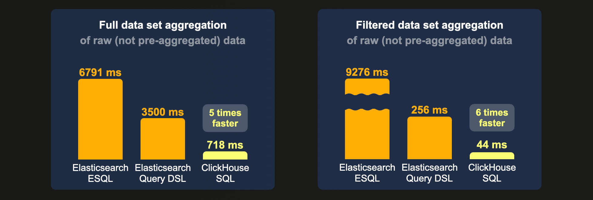
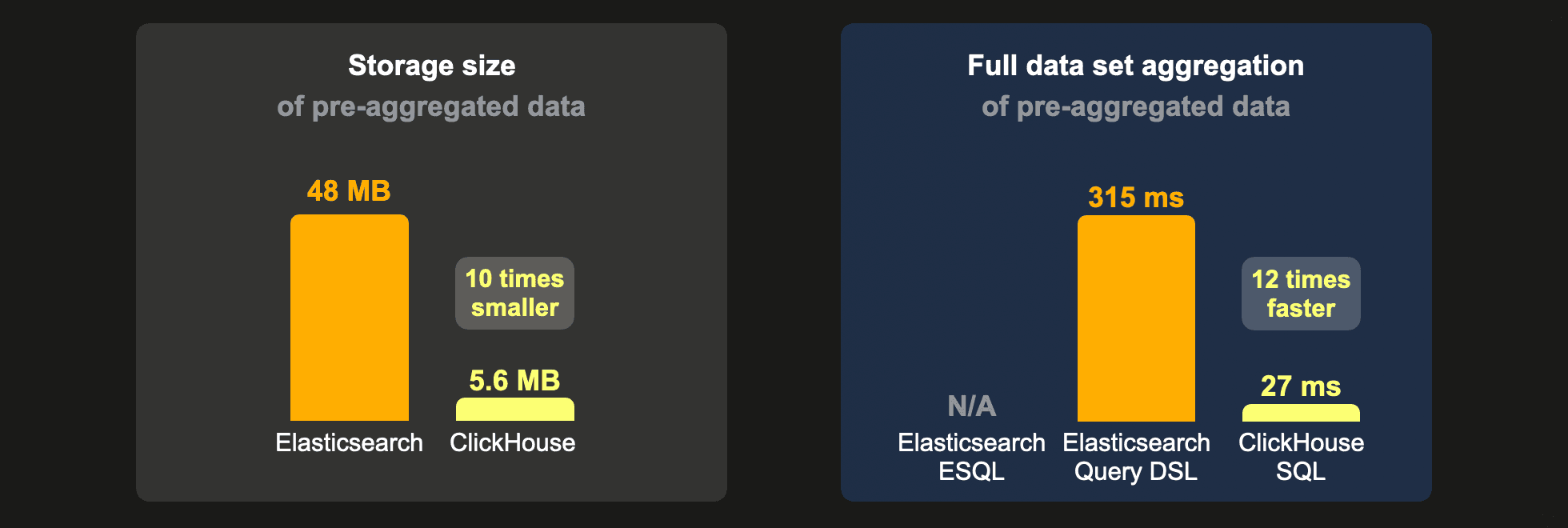
Count(*) aggregation queries in ClickHouse utilize hardware highly efficiently, resulting in at least 5 times lower latencies for aggregating large data sets compared to Elasticsearch. This requires smaller and 4 times cheaper hardware for comparable Elasticsearch latencies.

For these above-mentioned reasons, we increasingly see users migrating from Elasticsearch to ClickHouse, with customer stories highlighting:

• Highly reduced costs in petabyte-scale observability use cases:

“Migrating from Elasticsearch to ClickHouse, reduced the cost of our Observability hardware by over 30%.” Didi Tech

• Lifts in technical limitations of data analytics applications:

“This unleashed potential for new features, growth and easier scaling.” Contentsquare

• Drastic improvements in scalability and query latencies for monitoring platforms:

“ClickHouse helped us to scale from millions to billions of rows monthly.”
“After the switch, we saw a 100x improvement on average read latencies” The Guild

You will likely wonder, "Why is ClickHouse so much faster and more efficient than Elasticsearch?" This blog will give you an in-depth technical answer to this question.

A common use case for aggregation in data analytics scenarios is calculating and ranking the frequency of values in a dataset. As an example, all data visualizations in this screenshot from the ClickPy application (analyzing almost 900 billion rows of Python package download events) use a SQL GROUP BY clause in combination with a count(*) aggregation under the hood:

Similarly, in logging use cases (or more generally observability use cases), one of the most common applications for aggregations is to count how often specific log messages or events occur (and alerting in case the frequency is unusual).

The equivalent to a ClickHouse SELECT count(*) FROM ... GROUP BY ... SQL query in Elasticsearch is the terms aggregation, which is an Elasticsearch bucket aggregation.

ClickHouse’s GROUP BY with a count(*) and Elasticsearch’s terms aggregation are generally equivalent in terms of functionality, but they differ widely in their implementation, performance, and result quality, as described below.

We compare the performance of count aggregations in an accompanying blog post.

In addition to bucket aggregations, Elasticsearch also provides metric aggregations. We will leave a comparison of ClickHouse and Elasticsearch for metric use cases for another blog.

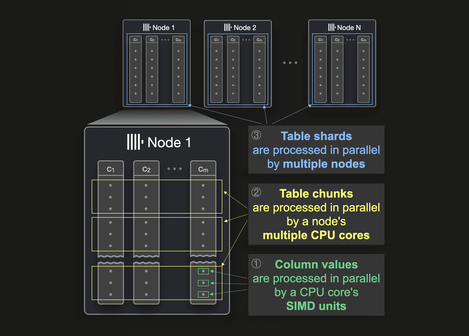
ClickHouse was built from the very beginning to filter and aggregate internet-scale data as quickly and efficiently as possible. To do so, ClickHouse parallelizes SELECT queries, including aggregation functions like count(*) and all other 90+ aggregation functions at the level of ① column values, ② table chunks, and ③ table shards:

ClickHouse utilizes the CPU's SIMD units (e.g. AVX512) to apply the same operations to consecutive values in a column. This blog post details how this works.

On a single machine with n CPU cores, ClickHouse runs an aggregation query with n parallel execution lanes (or fewer or more, if requested by the user via max_threads setting):

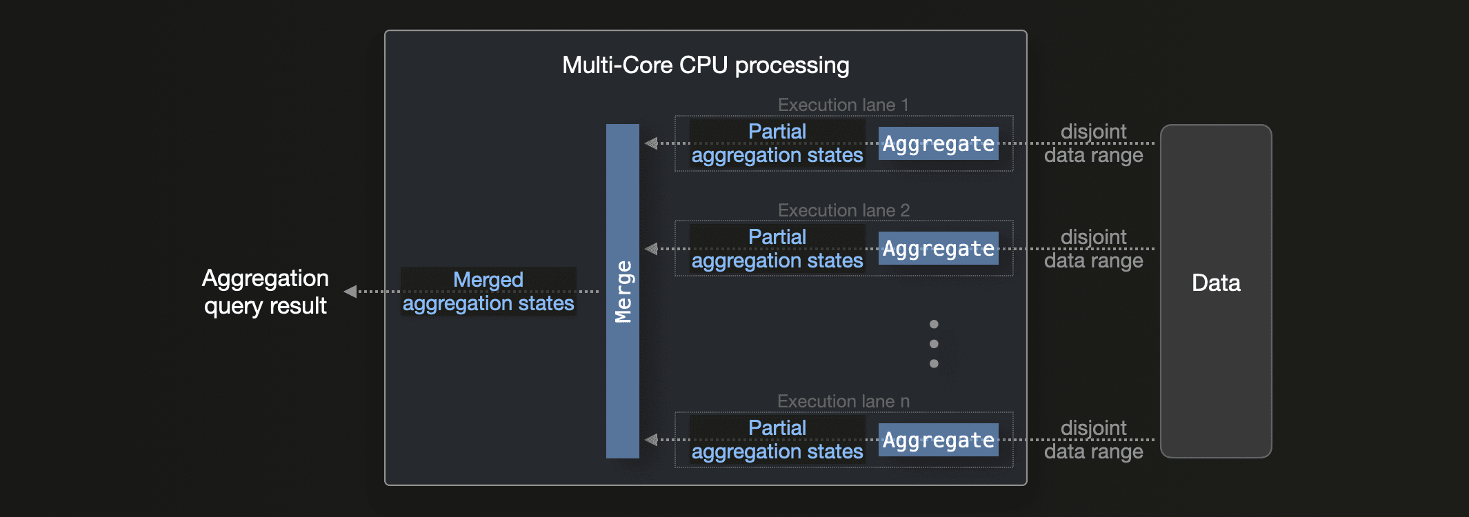
The figure above shows how ClickHouse processes n non-overlapping data ranges in parallel. These data ranges can be arbitrary, e.g. they don’t need to be based on the grouping key. When the aggregation query contains a filter in the form of a WHERE clause, and the primary index can be utilized to evaluate this filter, ClickHouse locates matching table data ranges and spreads these dynamically among the n execution lanes.

This parallelization approach is enabled using partial aggregation states: each of the n execution lanes produces partial aggregation states. These partial aggregation states are eventually merged into the final aggregation result.

For the count(*) aggregation, the partial aggregation state is simply an incrementally updated count variable. In fact, count(*) aggregation is the simplest kind of aggregation and could be parallelized internally, even without the concept of partial aggregation states. To give a concrete example where partial aggregation states enable parallelization, we use this aggregation query to calculate average house prices per town based on the UK property prices dataset:

SELECT
    town,
    avg(price) AS avg_price
FROM uk_price_paid
GROUP BY town;

Assume the database wants to calculate the average house prices in London using two parallel execution lanes:

Execution lane 1 averages the house prices of all rows in its data range consisting of two records for London. The resulting partial aggregation state for avg generally consists of

• a sum (here for execution lane 1: 500,000 as the summarized house prices in London) and
• a count (here for execution lane 1: 2 as the number of processed records for London).

Execution lane 2 calculates a similar partial aggregation state. These two partial aggregation states are merged, and with that, the final result can be produced: The average house price for the London records is (500,000 + 400,000) / (2 + 1) = 900,000 / 3 = 300,000.

Partial aggregation states are necessary to compute correct results. Simply averaging the averages of sub-ranges produces incorrect results. For example, if we average the average of the first sub-range (250,000) with the average of the second sub-range (400,000), we obtain (650,000 / 2) = 325,000, which is incorrect.

ClickHouse parallelizes all of its supported 90+ aggregation functions plus their combinations with aggregate function combinators across all available CPU cores.

If the source table of an aggregation query is sharded and spread over multiple nodes, then ClickHouse parallelizes aggregation functions across all available CPU cores of all available nodes.

Each node (in parallel) performs the aggregation locally using the aforementioned multi-core parallelization technique. The resulting partial aggregation states are streamed to and merged by the initiator node (the node that initially received the aggregation query):

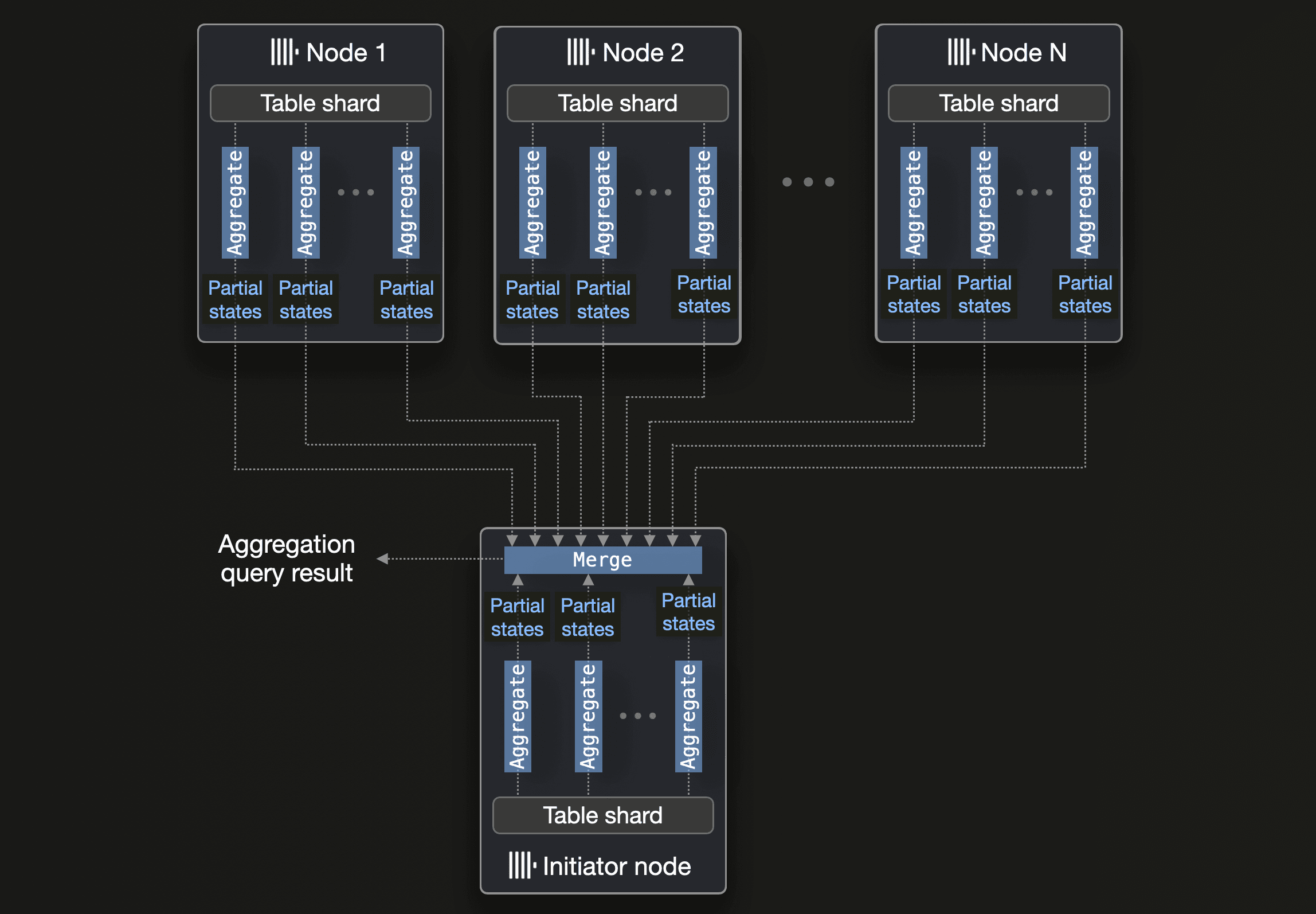
As an optimization, if the aggregation query’s GROUP BY key is a prefix of the sharding key, then the initiator node doesn’t need to merge partial aggregation states, and the merge happens as a last step on each node, and the final results are streamed back to the initiator node instead.

All techniques discussed so far are applied at "query time", i.e. when the user runs SELECT count(*) FROM ... GROUP BY ... queries. If the same expensive aggregation query is run repeatedly, e.g. hourly, or if sub-second latencies are required, but the queried data set is too large for that, then ClickHouse provides an additional optimization that shifts the load from the query time to the insert time and (mostly) the background merge time. Specifically, the above-mentioned partial aggregation technique (based on partial aggregation states) can also be used at the data part level during (parallel) background part merges.

This yields a powerful, highly scalable continuous data summarization technique, with the result that aggregation queries will find the majority of the data already aggregated. The following diagram sketches this:

① The -State aggregate function combinator can be used to instruct the ClickHouse query engine to only combine the partial aggregation states (produced by the parallel execution lanes) instead of combining and calculating the final result:

 SELECT
    town,
    avgState(price) AS avg_price_state
FROM uk_price_paid
GROUP BY town;

When you run this query, the partial aggregation states in avg_price_state are not really meant to be printed on the screen.

These combined partial aggregation states can then be written as data parts into a table with the AggregatingMergeTree table engine:

INSERT INTO <table with AggregatingMergeTree engine>
SELECT
    town,
    avgState(price) AS avg_price_state
FROM uk_price_paid
GROUP BY town;

② This table engine continues the partial aggregation incrementally (and parallelized) during background part merges. The merged result is the equivalent of running the aggregation query over all of the original data.

A materialized view does the insert step above automatically. Here's a concrete example based on the average house price per town example we used above.

③ At query time, the -Merge aggregate function combinator can be used to combine the partial aggregation states into the final result aggregation values:

SELECT
    town,
    avgMerge(avg_price_state) AS avg_price
FROM <table with AggregatingMergeTree engine>
GROUP BY town;

Compared with ClickHouse, Elasticsearch leverages a completely different parallelization approach for its terms aggregation (which is used to calculate counts in Elasticsearch). This leads to less efficient hardware utilization than ClickHous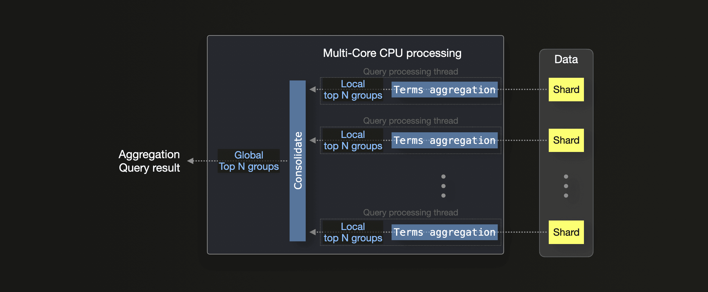e: The terms aggregation always needs a size parameter (called n in the following), and Elasticsearch runs this aggregation with one CPU thread per shard, independent of the number of CPU cores. Each thread calculates shard-local top n results (based on the largest count values per group by default) from its processed shard. Shard-local results are eventually consolidated into a global top n final result.

Elasticsearch’s multi-node parallelization of the terms aggregation works similarly. When the shards are spread over multiple nodes, each node produces (with the technique explained above) a node-local top n result, and these node-local results are consolidated into the final global result by the coordinating node (the node that initially received the aggregation query).

Based on how the data is spread over shards, this parallelization approach potentially has a precision issue. We illustrate this with an example: 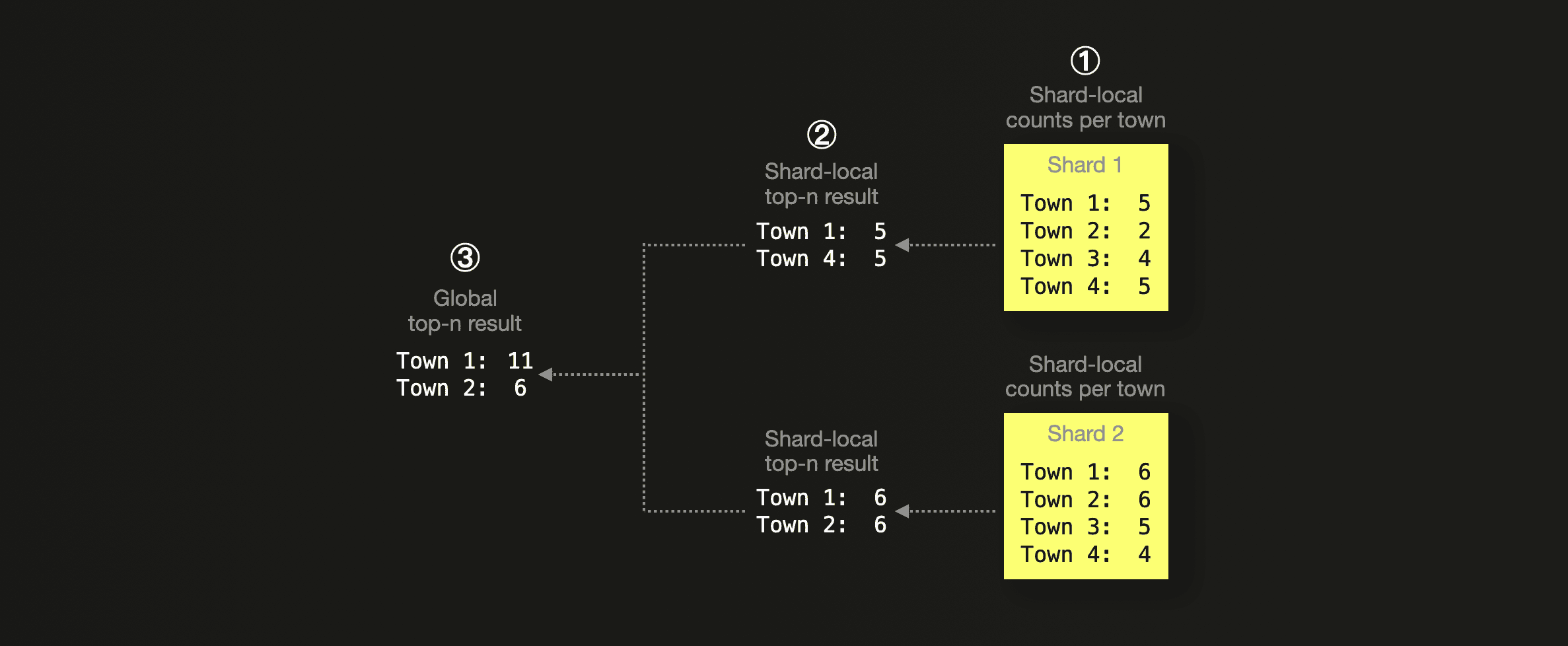We assume, based on the UK property prices dataset, that we want to calculate the top two towns with the most sold properties. The data is spread over two shards. The figure above shows abstractly ① the shard-local counts of property sale records per town. Each processing thread ② returns a shard-local top 2 result, which is consolidated ③ into the final global top 2 result. This result is incorrect, though. Based on the shard-global data, this is the correct count of records per town:

• Town 1: 11
• Town 2: 8
• Town 3: 9
• Town 4: 9

The ③ result calculated by Elasticsearch has both the count value and ranking for Town 2 wrong. Precision can be increased by analyzing returned count errors and adjusting the shard size parameter - this commands each processing thread to return a larger top n result from each shard than requested by the query, increasing memory requirements and runtimes.

Elasticsearch also leverages SIMD hardware units based on the JVM's auto-vectorization and the Java Panama Vector API. Additionally, since Elasticsearch 8.12 segments can be searched in parallel by query processing threads, with the exception of the terms aggregation. Because applying the above-mentioned technique to segments instead of shards has the same issue with precision. As a shard consists of multiple segments, this would also multiply the work per processing thread with an increased shard size parameter.

As described above, count values in Elasticsearch's terms aggregation are approximate by default when the queried data is split over more than one shard. The accuracy of results can be improved by analyzing returned count errors and adjusting the shard size parameter, but that increases runtimes and memory requirements.

The count(*) aggregation function in ClickHouse calculates fully accurate results.

ClickHouse count(*) aggregations are easy to use and don't require additional configuration like in Elasticsearch.

Because of its execution model, count aggregations without a limit clause are impossible in Elasticsearch — users must always specify a size setting. Even with large size values, bucket aggregations over high-cardinality data sets are restricted by the max_buckets setting or require paginating through results using an expensive composite aggregation.

ClickHouse count(*) aggregations are not limited by size restrictions. They additionally support spilling temporary results to disk if the query memory consumption exceeds an (optional) user-specified maximum memory threshold. In addition, independent of data set size, ClickHouse can run aggregations with minimal memory requirements if the grouping columns in an aggregation form a prefix of the primary key.

Again, ClickHouse count(*) aggregations have a lower degree of complexity compared to Elasticsearch.

No matter how efficient the aggregation and query processing in a database is, aggregating billions or trillions of rows (typical in modern data analytics use cases) will always be inherently costly due to the sheer amount of data that must be processed.

Therefore, databases specializing in analytical workloads often provide data summarization as a building block for users to automatically transform incoming data to a summarized data set, representing the original data in a pre-aggregated and usually significantly small format. Queries will utilize the precomputed data to provide sub-second latencies in interactive use cases, like the above-mentioned ClickPy application.

Both Elasticsearch and ClickHouse provide built-in techniques for automatic continuous data summarization. Their techniques have the same functional capabilities but drastically differ in implementation, efficiency, and with that, computing costs.

Elasticsearch provides a mechanism called transforms for batch-converting existing indices into summarized indices or continuously converting ingested data.

Based on the Elasticsearch on-disk format, we describe how transforms work here in detail.

We note three downsides of the Elasticsearch approach, namely:

• The requirement to retain old raw data: otherwise, transforms can’t correctly recalculate aggregations.

• Poor scalability and high computing costs: Whenever new raw data documents are detected for buckets after a checkpoint, all of the bucket data is queried from the ever-growing raw data source index and reaggregated. This doesn’t scale to billion, let alone trillion-scale document sets, and results in high computing costs.

• Not real-time: The transforms pre-aggregation target index is only up to date with the raw data source index after the next check interval.

Exclusively for time series metric data, Elasticsearch also provides a downsampling technique for reducing the footprint of that data by storing it at reduced granularity. Downsampling is the successor of rollups and equivalent to a transform that groups metrics data documents by their timestamp casted to a fixed time interval (e.g. hour, day, month, or year) and then applies a fixed set of aggregations ( min, max, sum, value_count, and average). A comparison with ClickHouse chained materialized views could be the topic of a future blog.

ClickHouse uses materialized views in combination with the AggregatingMergeTree table engine and partial aggregation states for automatic and (in contrast to Elasticsearch) incremental data transformation.

Based on ClickHouse’s on-disk format, we explain the mechanics of incremental materialized views in detail here.

ClickHouse materialized views have three key advantages over Elasticsearch transforms:

• No raw data dependency: Raw data in source tables is never queried, not even when the user wants to perform an exact aggregation calculation. This allows different TTL settings to be applied to the source and the pre-aggregated target table. Furthermore, in scenarios where only the same set of aggregation queries should be performed, users can choose to ditch the source data after pre-aggregation completely (using the Null table engine).

• High scalability and low computing costs: Incremental aggregation is engineered especially for scenarios where raw data source tables contain billions or trillions of rows. Instead of querying the ever-growing source table repeatedly and recalculating aggregate values from all existing rows belonging to the same group when new raw data rows for that group exist, ClickHouse simply calculates a partial aggregation state from (only) the values of the newly inserted raw data rows. This state is incrementally merged with the previously calculated states in the background. In other words - each raw data value is aggregated with other raw data values exactly once. This results in dramatically lower computing costs compared to aggregation by brute force over the raw data.

• Real-time: When an insert into the raw data source table is successfully acknowledged, the pre-aggregation target table is guaranteed to be up-to-date.

In our accompanying benchmark blog post, we use continuous transforms in Elasticsearch and equivalent materialized views in ClickHouse to pre-aggregate ingested data on the fly into separate data sets. Sometimes, this is not feasible. For example, when a large portion of the data is already ingested, re-ingesting is not possible or too expensive, and queries that would benefit from running over this data in a pre-aggregated format are introduced.

We simulated this scenario in Elasticsearch by running a batch transform over the already ingested 10 billion rows data set, pre-calculating counts into a separate data set to speed up an aggregation query that we use as part of our benchmark. Both continuous and batch transforms use the same checkpoints-based mechanism described above. Because of the downsides of this mechanism, where the same values are queried and aggregated repeatedly at checkpoints:

Backfilling via the batch transform took 5 full days (using significant computing costs). It is a long time to wait until queries can benefit from the pre-aggregated data.

In ClickHouse, backfilling pre-aggregations works by using an INSERT INTO SELECT statement to insert directly into the materialized view’s target table using the view's SELECT query (transformation) :

For the 10 billion rows data set, this takes 20 seconds instead of 5 full days.

These 20 seconds include aggregating the full 10 billion row data set and writing the result (as partial aggregation states) into the target table, which will be used subsequently for the materialized view to handle additional incoming data. Depending on the cardinality of the raw data set, this can be a memory-intensive approach, as the complete raw data set is ad-hoc aggregated. Alternatively, users can utilize a variant that requires minimal memory.

Note that the 20 seconds ClickHouse approach of manually aggregating the raw data set and directly inserting the result into the target table is not feasible in Elasticsearch. Theoretically, this could work with a reindex (index to index copy) operation. However, this would require keeping the _source data in the raw data set (requiring drastically more storage space). It would also require a mechanism to manually create the necessary checkpoints to correctly continue the pre-aggregation process when streaming data starts. In ClickHouse, the materialized views will just continue with the incremental aggregation process for new incoming data after we run the backfilling as described above.

Most databases, including ClickHouse, implement GROUP BY using some variant of the hash aggregation algorithm in which the aggregation values of input rows are stored and updated in a hash table with the grouping columns as key. Choosing the right kind of hash table is critical for performance. Under the hood, ClickHouse utilizes a sophisticated hash table framework to implement aggregations. Depending on the data type of the grouping columns, the estimated cardinality, and other factors, the fastest hash table is selected individually for each aggregation query from over 30 (as of April 2024) different implementations. ClickHouse was purposely built for high-performance aggregations over vast data amounts.

ClickHouse is today amongst the fastest databases on the market, with distinctive features for data analytics:

• State-of-the-art vectorized query engine with parallelized execution across all server and cluster resources, utilizing hardware up to the theoretical limits

• Modern SQL dialect and rich data types, including maps and arrays (plus over 80 functions for working with arrays) for modeling and solving a wide range of problems elegantly and simply

• Over 90 pre-built aggregation functions with support for incremental aggregation of large data sets, plus powerful aggregation combinators for extending the behavior of other aggregation functions

• Over 1000 regular data processing functions for domains like mathematics, geo, machine learning, time series, and more

• Fully parallelized window functions

• Parallel join algorithms

• Native support for loading data in 90+ file formats from virtually any data source

In this blog post, we provided an in-depth technical answer to the question of why ClickHouse is so much faster and more efficient than Elasticsearch for processing count aggregations, which are commonly needed in data analytics and logging/observability use cases.

We explained parallelization approaches and the difference in result quality and usability complexity of count aggregations in ClickHouse and Elasticsearch. We explored Elasticsearch and ClickHouse's built-in mechanisms for pre-calculating counts. We highlighted why ClickHouse materialized views are much more efficient and better suited for processing billion/trillion-scale row sets than Elasticsearch transforms.

We suggest reading our accompanying blog post ClickHouse vs. Elasticsearch: The Billion-Row Matchup to see ClickHouse high-performance aggregations in action. As a teaser, we include some of the benchmark results here: