Another month goes by, which means it’s time for another release!
ClickHouse version 24.7 contains 18 new features 🎁 12 performance optimisations 🛷 76 bug fixes 🐛
New Contributors #
As always, we send a special welcome to all the new contributors in 24.7! ClickHouse's popularity is, in large part, due to the efforts of the community that contributes. Seeing that community grow is always humbling.
Below are the names of the new contributors:
0x01f, AntiTopQuark, Daniel Anugerah, Elena Torró Martínez, Filipp Bakanov, Gosha Letov, Guspan Tanadi, Haydn, Kevin Song, Linh Giang, Maksim Galkin, Max K., Nathan Clevenger, Rodolphe Dugé de Bernonville, Tobias Florek, Yinzuo Jiang, Your Name, Zawa-II, cw5121, gabrielmcg44, gun9nir, jiaosenvip, jwoodhead, max-vostrikov, maxvostrikov, nauu, 忒休斯~Theseus
Hint: if you’re curious how we generate this list… click here.
You can also view the slides from the presentation.
Optimizations for reading in order #
Contributed by Anton Popov #
When reading data from tables, ClickHouse applies some optimizations by default. One of these optimizations is optimize_read_in_order: If a query’s ORDER BY columns form a prefix of the table’s primary key, or if in a full sorting merge join the physical row order of one or both joined tables matches the join key sort order, the data can be read in disk order, and the sorting operation can be skipped. This is also generally beneficial for memory usage. Less memory is required as no full in-memory sort takes place. In addition, short-circuiting is possible when the query uses a LIMIT clause.
The optimize_read_in_order optimization prevents data from being re-sorted but reduces the parallelism for reading the table data. Normally, the table data is split into non-overlapping ranges read (streamed) by N threads in parallel into the query engine for further processing (N is controlled by the max_threads setting).
The following diagram shows why this approach is not feasible for the optimize_read_in_order optimization:
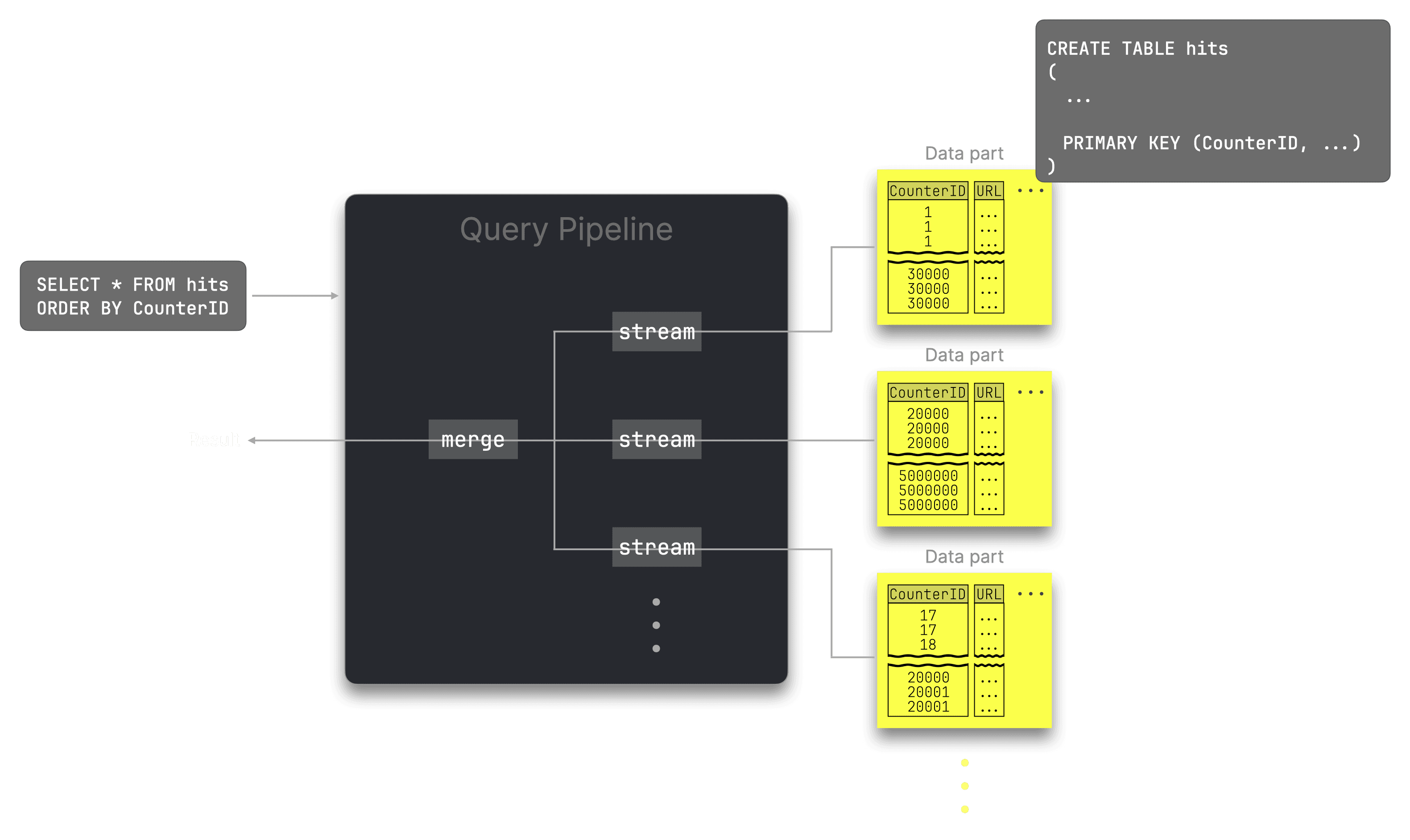
In the diagram above, we sketch some data parts belonging to a table whose rows on disk are sorted (per data part) by the CounterID column first. We show the query pipeline (the physical execution plan) executing a query that contains an ORDER BY clause matching the table’s physical on-disk order of rows. Therefore, there is no need to re-sort the data. Instead, the already (locally) sorted rows from the table’s data parts are merged by interleaved linear scans within and across the data parts. This means that the data is not streamed concurrently but sequentially.
ClickHouse 24.7 now introduces buffering of the table part’s data before the merge step, controlled by the setting read_in_order_use_buffering (enabled by default). It increases the memory usage but also increases the parallelism of query execution because it allows streaming the data into the buffer concurrently before this data is merged into the final result:
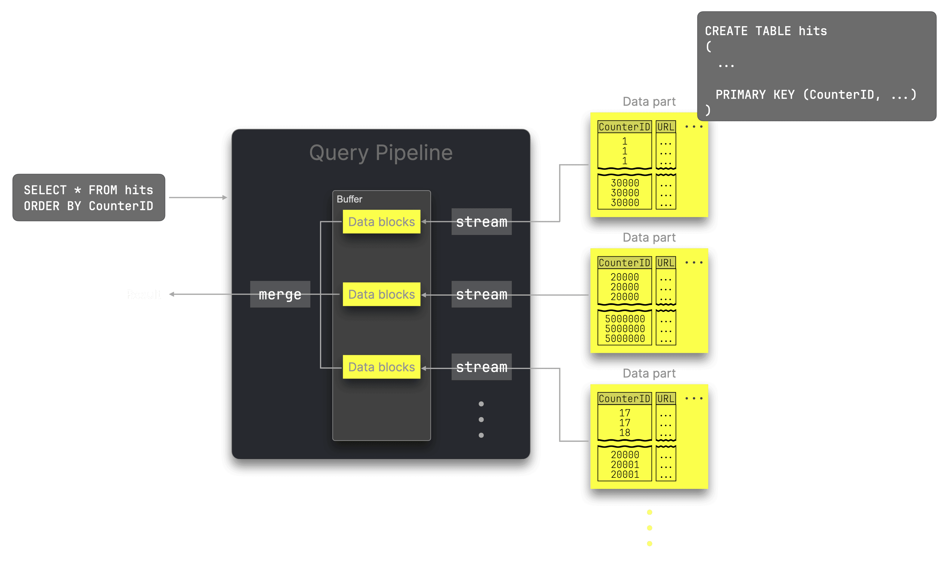
This increases the performance of queries with applied optimize_read_in_order optimization up to 10x if the query uses a high-selectivity filter (which greatly reduces the amount of data being streamed and buffered).
Let’s see it in action with help from the Anonymized Web Analytics Data dataset, which consists of 100 million anonymized page hits. ClickBench also uses this dataset, and we can create the table using the provided DDL statement.
Note that the table has the following primary key:
PRIMARY KEY (CounterID, EventDate, UserID, EventTime, WatchID)
Next, we insert the data:
INSERT INTO hits SELECT * FROM s3('s3://clickhouse-public-datasets/hits_compatible/hits.parquet');
We loaded this dataset onto a ClickHouse instance running on an AWS c6a.8xlarge instance.
Let’s start by writing a query that doesn’t use the new buffering approach (note that we disabled the file system cache to better compare this and the next query run):
SELECT
    CounterID,
    UserID
FROM hits_100m_obfuscated
WHERE RegionID = 2
ORDER BY CounterID ASC
FORMAT `Null`
SETTINGS enable_filesystem_cache = 0,
         read_in_order_use_buffering = 0

0 rows in set. Elapsed: 0.590 sec. Processed 100.00 million rows, 1.58 GB (169.48 million rows/s., 2.67 GB/s.)
Peak memory usage: 17.82 MiB.
This query takes around 0.6 seconds and uses 18 MB of memory. Now, let’s enable buffering:
SELECT
    CounterID,
    UserID
FROM hits_100m_obfuscated
WHERE RegionID = 2
ORDER BY CounterID ASC
FORMAT `Null`
SETTINGS enable_filesystem_cache = 0,
         read_in_order_use_buffering = 1


0 rows in set. Elapsed: 0.097 sec. Processed 100.00 million rows, 1.58 GB (1.04 billion rows/s., 16.35 GB/s.)
Peak memory usage: 48.37 MiB.
The query time is reduced to under 0.1 seconds, and the memory usage is 48 MB. So, the buffering feature has sped this query up 5 times while using 3 times the memory.
Faster parallel Hash Join #
Contributed by Nikita Taranov #
Every ClickHouse release comes with JOIN improvements.
In this release, we improved the allocation of hash tables for the parallel hash join algorithm.
As a reminder, the parallel hash join algorithm is a variation of a hash join that splits the input data to build several hash tables concurrently, speeding up the build phase at the expense of higher memory overhead.
The default hash join algorithm requires less memory than the parallel hash join algorithm by using a single hash table to fill the data from the right-hand side table of the JOIN. For this, the right-hand side table’s data can be split and read in parallel by multiple threads, but only a single thread can fill this data into the hash table, as hash tables are not thread-safe for insertions. This can become a bottleneck for the JOIN runtime if the right-hand side table is large.
The following diagram shows how the parallel hash join algorithm overcomes this bottleneck:
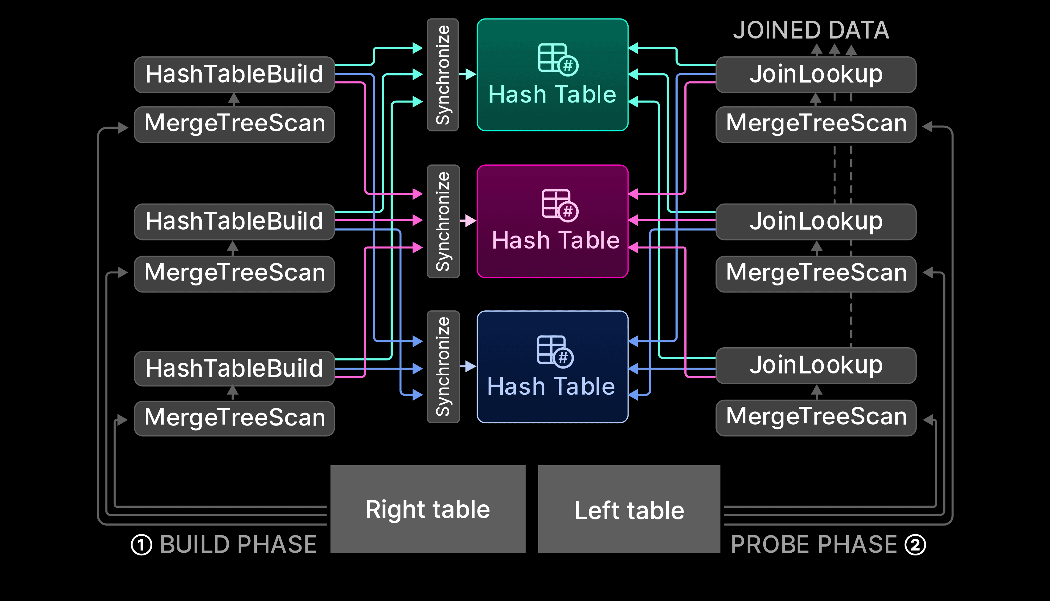
In the algorithm’s ① build phase, the data from the right table is split and streamed in parallel by N streams (N is controlled by the max_threads setting) to fill N hash tables in parallel. The rows from each stream are routed to one of the N hash tables by applying a hash function to the join keys of every row. The hash function for splitting the rows into hash tables differs from the one used internally in the hash tables.
In the algorithm’s ② probe phase, data from the left table is split and streamed in parallel by N streams (again, N is controlled by the max_threads setting). The same ‘bucket hash function’ from step ① is applied to the join keys of each row to determine the corresponding hash table, and the rows are joined by doing lookups into the corresponding hash table.
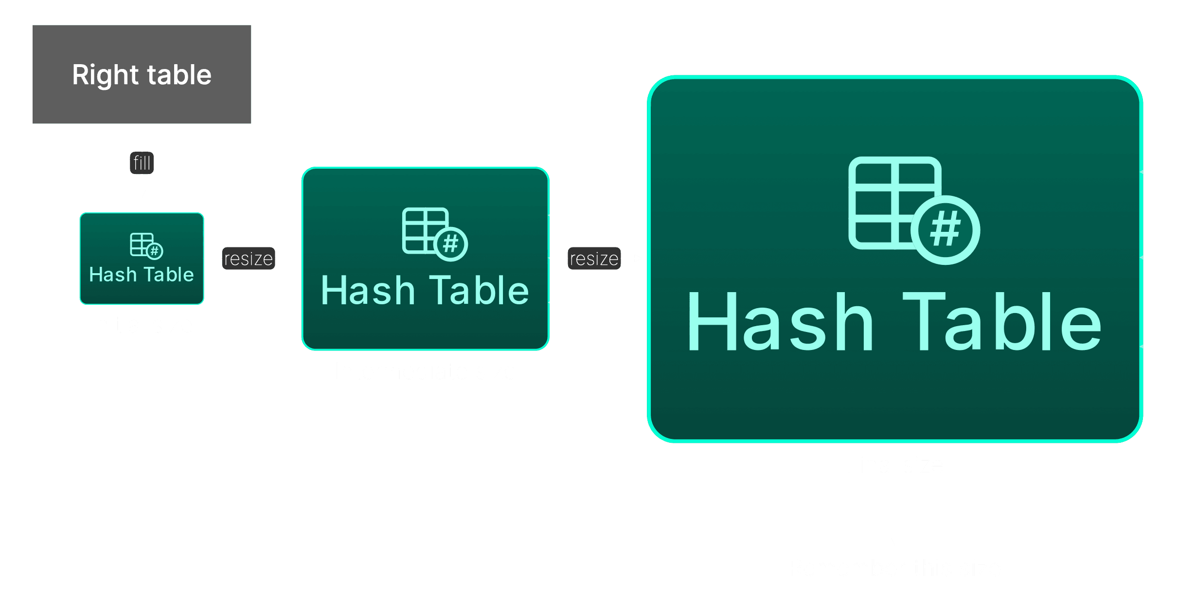
To avoid wasting memory, hash tables are pre-allocated with a limited initial size. If a table runs full, a new larger hash table is allocated, data from the previous table is copied over, and the old table is deallocated. The larger size of the new hash table is always chosen by increasing the size of the previous table with an internal multiplier.
In ClickHouse 24.7, when a parallel hash join is finished, the final sizes of hash tables are now collected and cached (with the JOIN’s right table name and names of the join columns used as input for the lookup key). In subsequent query executions, hash tables are pre-allocated based on their remembered size from previous query runs. This saves time by avoiding redundant intermediate resize steps. The next diagram visualizes this:
Let’s demonstrate this with a concrete example.
We use the ClickBench table, which contains 100 million anonymized page hits.
First, we create the table by running the provided DDL statement. Next, we insert the data:
INSERT INTO hits SELECT * FROM s3('s3://clickhouse-public-datasets/hits_compatible/hits.parquet');
After the data load, the table should contain ~100 million rows:
SELECT count()
FROM hits;

   ┌──count()─┐
1. │ 99997497 │ -- 100.00 million
   └──────────┘
We run a JOIN query performing a self-join. Note that this JOIN is using the hash join algorithm by default:
SELECT count()
FROM hits AS t1
INNER JOIN hits AS t2 ON t1.ClientIP = t2.RemoteIP
WHERE t1.ClientIP != 0;

   ┌─count()─┐
1. │ 3395861 │ -- 3.40 million
   └─────────┘

1 row in set. Elapsed: 5.112 sec. Processed 199.99 million rows, 799.98 MB (39.12 million rows/s., 156.49 MB/s.)
Peak memory usage: 3.25 GiB.
Now we run the same JOIN query with the parallel hash join algorithm:
SELECT count()
FROM hits AS t1
INNER JOIN hits AS t2 ON t1.ClientIP = t2.RemoteIP
WHERE t1.ClientIP != 0
SETTINGS join_algorithm = 'parallel_hash';

   ┌─count()─┐
1. │ 3395861 │ -- 3.40 million
   └─────────┘

1 row in set. Elapsed: 0.517 sec. Processed 199.99 million rows, 799.98 MB (387.03 million rows/s., 1.55 GB/s.)
Peak memory usage: 3.44 GiB.
Note that this query runs 10 times faster on the same hardware.
When we run the query for the first time since the ClickHouse process got started, with the parallel hash join algorithm and enabled trace-level logging, then we can observe log messages indicating that ClickHouse is collecting and caching hash table size statistics:
SELECT count()
FROM hits AS t1
INNER JOIN hits AS t2 ON t1.ClientIP = t2.RemoteIP
WHERE t1.ClientIP != 0
SETTINGS
  join_algorithm = 'parallel_hash',
  send_logs_level = 'trace';

...
<Trace> HashTablesStatistics: Statistics updated for key=18113390195926062714: new sum_of_sizes=9594872, median_size=149909
...
When we rerun the query (without any restart of the ClickHouse process in between) with enabled trace-level logging, we can observe how ClickHouse is accessing the cached hash table statistics before pre-allocations.
SELECT count()
FROM hits AS t1
INNER JOIN hits AS t2 ON t1.ClientIP = t2.RemoteIP
WHERE t1.ClientIP != 0
SETTINGS
  join_algorithm = 'parallel_hash',
  send_logs_level = 'trace';

...
<Trace> HashTablesStatistics: An entry for key=18113390195926062714 found in cache: sum_of_sizes=9594872, median_size=149909
...
Merge Join algorithm for ASOF JOIN #
Contributed by Vladimir Cherkasov #
ClickHouse was the first SQL DBMS to introduce the ASOF JOIN in April 2019.
As a reminder, ASOF JOIN provides non-exact matching capabilities. If a row from the left table doesn’t have an exact match in the right table, then the closest matching row from the right table is used as a match instead.
This is particularly useful for time-series analytics and can drastically reduce query complexity.
Also, when ClickHouse is used as a feature store for machine learning, the ASOF JOIN is handy. It allows to easily combine the features appropriately to produce a set of feature vectors.
So far, ASOF JOIN only supported the memory-bound hash and parallel hash join algorithms.
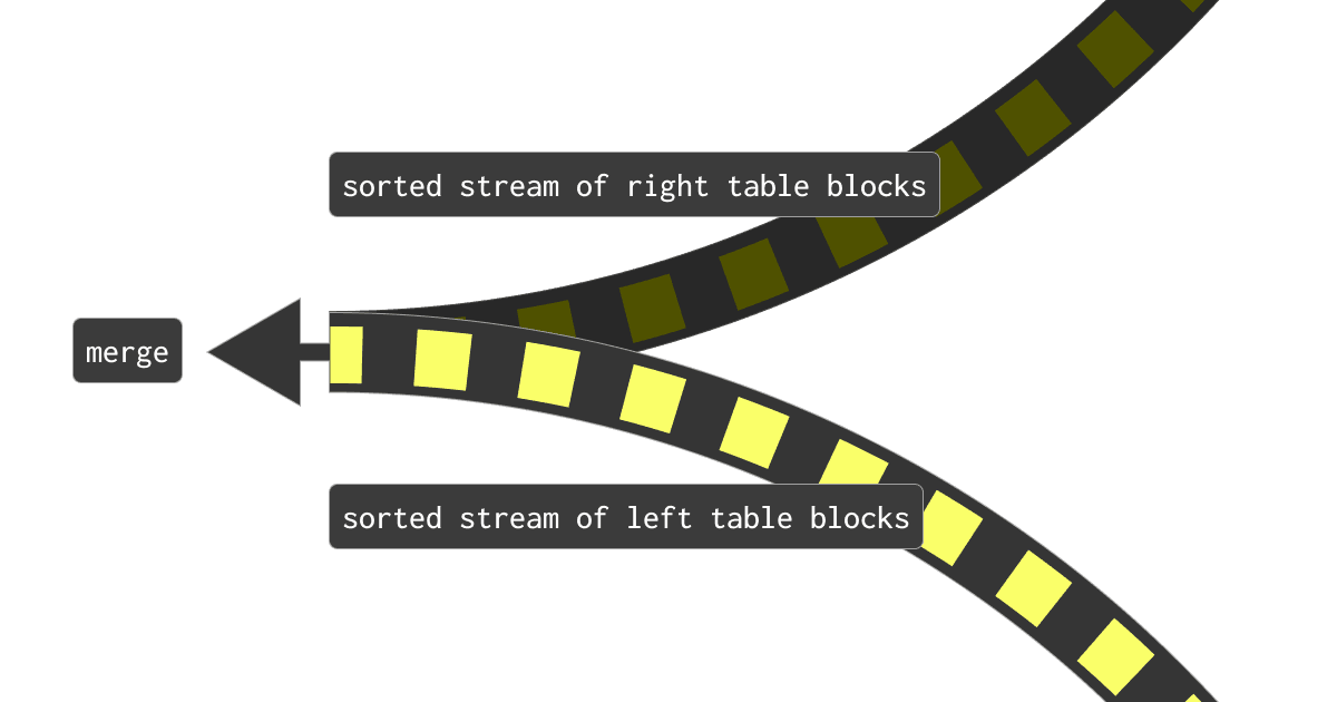
Since ClickHouse 24.7 ASOF JOIN also works with the non-memory bound full sorting merge join algorithm. As a reminder, the join strategy of that algorithm requires the joined data to first be sorted in order of the join keys before join matches can be identified by interleaved linear scans and merges of the sorted streams of blocks of rows from both tables:
The full sorting merge join can take advantage of the physical row order of one or both tables, allowing sorting to be skipped (plus benefiting from the new optimizations for reading in order, described in a section further above). In such cases, the join performance can be competitive with the hash join algorithms, while generally requiring significantly less memory. Otherwise, the full sorting merge join needs to fully sort the rows of the tables before identifying join matches. The sorting can occur in memory, and the memory usage generally is independent of the size of the joined tables.
Let’s look at a concrete example.
Imagine that we are tracking internet user’s website click events in a hits table and user sessions in a sessions table. Then, we can use ASOF JOIN to concisely formulate a query for finding the first user click event for each session:
SELECT ...
FROM hits h ASOF JOIN sessions s
ON h.UserID = s.UserID AND h.EventTime > s.StartTime;
We are simulating the sessions table with the hits table and reformulate the query from above to a self ASOF JOIN:
SELECT ...
FROM hits t1 ASOF JOIN hits t2
ON t1.UserID = t2.UserID AND t1.EventTime < t2.EventTime;
To run this query, we create the hits table using the DDL statement provided by ClickBench.
Next, we insert the data (100 million rows):
INSERT INTO hits SELECT * FROM s3('s3://clickhouse-public-datasets/hits_compatible/hits.parquet');
Now we are ready to run the ASOF join query from above with the default hash join algorithm:
SELECT count()
FROM hits t1 ASOF JOIN hits t2
ON t1.UserID = t2.UserID AND t1.EventTime < t2.EventTime;

   ┌──count()─┐
1. │ 81878322 │ -- 81.88 million
   └──────────┘

1 row in set. Elapsed: 11.849 sec. Processed 199.99 million rows, 2.40 GB (16.88 million rows/s., 202.55 MB/s.)
Peak memory usage: 6.49 GiB.
Let’s run the same query with the full sorting merge join algorithm instead:
SELECT count()
FROM hits t1 ASOF JOIN hits t2
ON t1.UserID = t2.UserID AND t1.EventTime < t2.EventTime
SETTINGS
    join_algorithm = 'full_sorting_merge';

   ┌──count()─┐
1. │ 81878322 │ -- 81.88 million
   └──────────┘

1 row in set. Elapsed: 5.041 sec. Processed 199.99 million rows, 2.40 GB (39.68 million rows/s., 476.11 MB/s.)
Peak memory usage: 2.41 GiB.
As you can see, for our specific data set, the ASOF join implemented by the full sorting merge join algorithm runs over two times faster and consumes over two times less peak main memory than the ASOF join run with the hash join algorithm. However, this is not a general rule, and it’s best to test it with your specific data sets.
percent_rank #
Contributed by lgbo-ustc #
The percent_rank returns the relative rank (i.e., percentile) of rows within a window partition.
Let’s look at how it works with help from a synthetic dataset of soccer player salaries. We’ll create a table called salaries:
CREATE TABLE salaries
ORDER BY team AS
SELECT *
FROM url(
'https://raw.githubusercontent.com/ClickHouse/examples/main/LearnClickHouseWithMark/WindowFunctions-Ranking/data/salaries.csv'
)
SETTINGS schema_inference_make_columns_nullable=0;
Then, we can compute the rank and percent_rank of those salaries:
SELECT
    team, player, weeklySalary AS salary, position AS pos,
    rank() OVER (ORDER BY salary DESC) AS rank,
    round(percent_rank() OVER (ORDER BY salary DESC), 6) AS percentRank
FROM salaries
ORDER BY salary DESC
LIMIT 10
┌─team─────────────────────────┬─player──────────┬─salary─┬─pos─┬─rank─┬─percentRank─┐
│ North Pamela Trojans         │ Robert Griffin  │ 399999 │ GK  │    1 │           0 │
│ Jimmyville Legionnaires      │ Nathan Thompson │ 399998 │ D   │    2 │    0.000004 │
│ Stephaniemouth Trojans       │ Benjamin Cline  │ 399998 │ D   │    2 │    0.000004 │
│ Maryhaven Generals           │ Scott Chavez    │ 399998 │ M   │    2 │    0.000004 │
│ Michaelborough Rogues        │ Dan Conner      │ 399998 │ M   │    2 │    0.000004 │
│ Nobleview Sages              │ William Rubio   │ 399997 │ M   │    6 │     0.00002 │
│ North Christinaview Archers  │ Robert Cook     │ 399991 │ M   │    7 │    0.000024 │
│ North Krystal Knights-Errant │ Juan Bird       │ 399986 │ GK  │    8 │    0.000028 │
│ Claireberg Vikings           │ Benjamin Taylor │ 399985 │ M   │    9 │    0.000032 │
│ Andreaberg Necromancers      │ John Lewis      │ 399985 │ D   │    9 │    0.000032 │
└──────────────────────────────┴─────────────────┴────────┴─────┴──────┴─────────────┘
Automatic named tuples #
Contributed by Amos Bird #
A named tuple will be created if you specify aliases (using AS) for tuple elements. Let’s have a look at how this used to work in 24.6:
docker run --rm clickhouse/clickhouse-server:24.6 \
  clickhouse-local \
  --query \
  "SELECT ('Hello' AS a, 123 AS b) AS x,
          toTypeName(x) AS type,
          toJSONString(x) AS json
   FORMAT Vertical"
Row 1:
──────
x:    ('Hello',123)
type: Tuple(String, UInt8)
json: ["Hello",123]
And now, 24.7:
docker run --rm clickhouse/clickhouse-server:24.7 \
  clickhouse-local \
  --query \
  "SELECT ('Hello' AS a, 123 AS b) AS x,
          toTypeName(x) AS type,
          toJSONString(x) AS json
   FORMAT Vertical"
Row 1:
──────
x:    ('Hello',123)
type: Tuple(
    a String,
    b UInt8)
json: {"a":"Hello","b":123}


