Table of Contents
Introduction
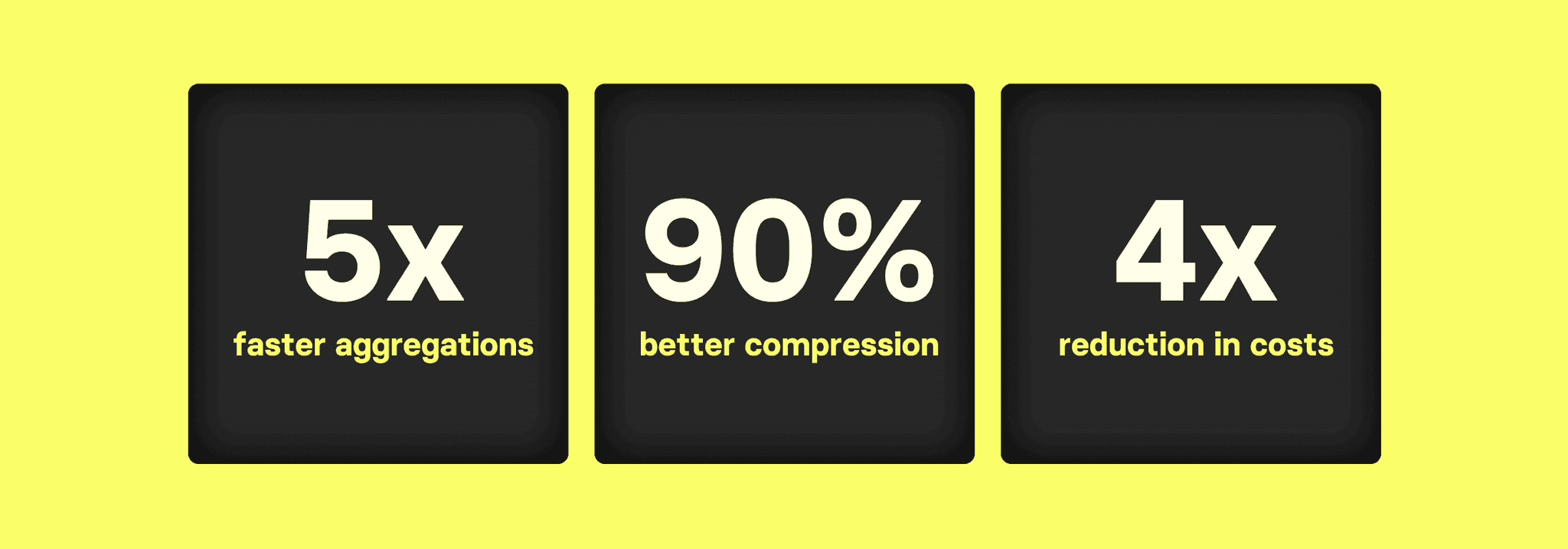
This blog examines the performance of ClickHouse vs. Elasticsearch for workloads commonly present in large-scale data analytics and observability use cases – count(*) aggregations over billions of table rows. This type of analysis is fundamental to many time-series database workloads, where understanding event frequency over time is critical. It shows that ClickHouse vastly outperforms Elasticsearch for running aggregation queries over large data volumes. Specifically:
- ClickHouse compresses data much better than Elasticsearch, resulting in 12 to 19 times less storage space for large data sets, allowing smaller and cheaper hardware to be used.

Count(*)aggregation queries in ClickHouse utilize hardware highly efficiently, resulting in at least 5 times lower latencies for aggregating large data sets compared to Elasticsearch. This requires smaller and, as we will demonstrate later, 4 times cheaper hardware for comparable Elasticsearch latencies.
- ClickHouse features a much more storage- and compute-efficient continuous data summarization technique – ClickHouse materialized views vs Elasticsearch transforms, further lowering computing and storage costs.
For these above-mentioned reasons, we increasingly see users migrating from Elasticsearch to ClickHouse, with customers highlighting:
“Migrating from Elasticsearch to ClickHouse, reduced the cost of our Observability hardware by over 30%.” Didi Tech
- Lifts in technical limitations of data analytics applications:
“This unleashed potential for new features, growth and easier scaling.” Contentsquare
- Drastic improvements in scalability and query latencies for monitoring platforms:
“ClickHouse helped us to scale from millions to billions of rows monthly.”
“After the switch, we saw a 100x improvement on average read latencies” The Guild
In this post, we will compare storage sizes and count(*) aggregation query performance for a typical data analytics scenario. To keep the scope suitable for one blog, we will compare the single-node performance of running count(*) aggregation queries in isolation over large data sets.
The rest of this blog first motivates why we focussed on benchmarking count(*) aggregations. We then describe the benchmark setup and explain our count(*) aggregation performance test queries and benchmark methodology. Finally, we will present the benchmark results.
While reading the benchmark results, you will likely wonder, "Why is ClickHouse so fast and efficient?" The short answer is attention to a myriad of details for how to optimize and parallelize large-scale data storage and aggregation execution. We suggest reading ClickHouse vs. Elasticsearch: The Mechanics of Count Aggregations for an in-depth technical answer to this question.
Count aggregations in ClickHouse and Elasticsearch
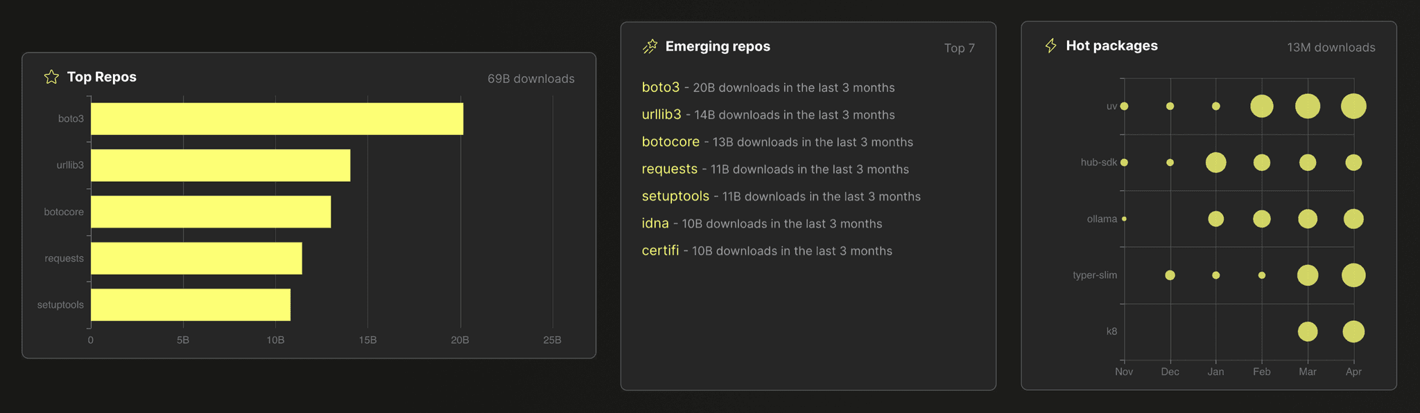
A common use case for aggregation in data analytics scenarios is calculating and ranking the frequency of values in a dataset. As an example, all data visualizations in this screenshot from the ClickPy application (analyzing almost 900 billion rows of Python package download events) use a SQL GROUP BY clause in combination with a count(*) aggregation under the hood:
Similarly, in logging use cases (or more generally observability use cases), one of the most common applications for aggregations is to count how often specific log messages or events occur (and alerting in case the frequency is unusual).
The equivalent to a ClickHouse SELECT count(*) FROM ... GROUP BY ... SQL query in Elasticsearch is the terms aggregation, which is an Elasticsearch bucket aggregation.
We describe how Elasticsearch and ClickHouse process such count aggregations under the hood in an accompanying blog post. In this post, we will compare the performance of these count(*) aggregations.
Benchmark setup
Data
We are going to use the public PyPI download statistics data set. Each row in this (constantly growing) data set represents one download of a Python package by a user (using pip or a similar technique). Last year, my colleague Dale built the above-mentioned analytics application on top of that data set analyzing almost 900 billion rows (as of May 2024) in real-time, powered by ClickHouse aggregations.
We use a version of this data set hosted as Parquet files in a public GCS bucket.
From this bucket, we will load 1, 10, and 100* billion rows into Elasticsearch and ClickHouse to benchmark the performance of typical data analytics queries.
*We were unable to load the
100 billion row raw dataset into Elasticsearch.
Hardware
This blog focuses on single-node data analytics performance. We leave benchmarks of multi-node setups for future blogs.
We use a single dedicated AWS c6a.8xlarge instance for both Elasticsearch and ClickHouse. This has 32 CPU cores, 64 GB RAM, a locally attached SSD with 16k IOPS, and Ubuntu Linux as the OS.
Additionally, we compare the performance of a ClickHouse Cloud service consisting of nodes with similar specifications regarding the number of CPU cores and RAM.
Data loading setup
We load the data from Parquet files hosted in a GCS bucket:
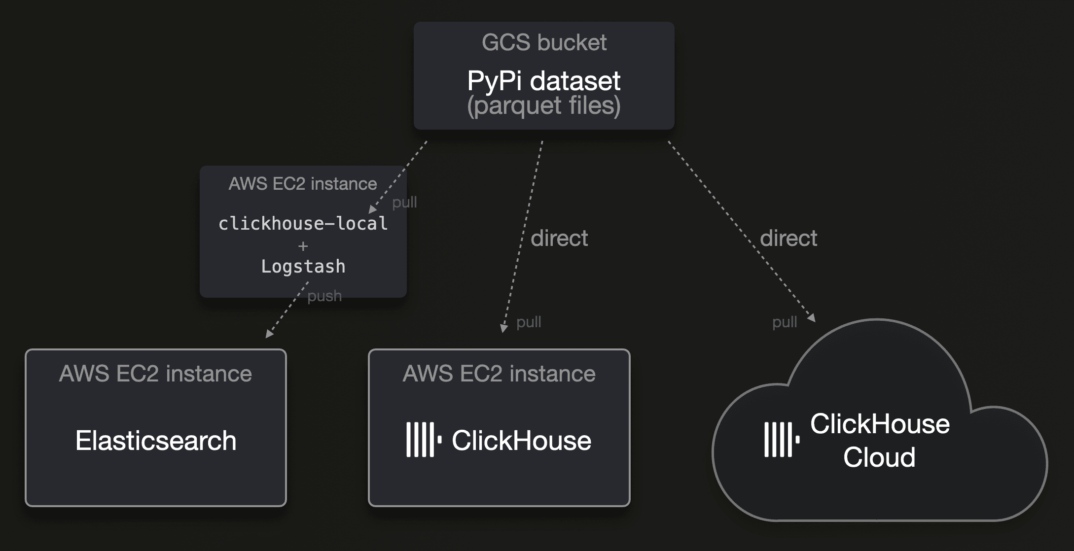
Parquet is increasingly becoming the ubiquitous standard for distributing analytics data in 2024. While this is supported out-of-the-box by ClickHouse, Elasticsearch has no native support for this file format. Logstash, its recommended ETL tool, additionally has no support for this file format at the time of writing.
Elasticsearch
To load the data into Elasticsearch, we use clickhouse-local and Logstash. Clickhouse-local is the ClickHouse database engine turned into a (blazingly fast) command line utility. The ClickHouse database engine natively supports 90+ file formats and provides 50+ integration table functions and engines for connectivity with external systems and storage locations, meaning that it can read (pull) data in almost any format from virtually any data source. Out of the box. And highly parallel. Because ClickHouse is a relational database engine, we can utilize all of what SQL offers to filter, enrich, and transform this data on the fly with clickhouse-local before sending it to Logstash. This is the configuration file used for Logstash, and this is the command line call driving the data load into Elasticsearch.
We could have utilized the ClickHouse url table function for sending the data directly to Elasticsearch’s REST API with clickhouse-local. However, Logstash allows easier tuning of batching and parallelism settings, supports sending data to multiple outputs (e.g. multiple Elasticsearch data streams with different settings), and has built-in resiliency, including backpressure and retries of failed batches with intermediate buffering and dead letter queues.
ClickHouse
Because, as mentioned above, ClickHouse can natively read Parquet files from object storage buckets of most cloud providers, we simply used this SQL insert statement to load the data into ClickHouse and ClickHouse Cloud. For ClickHouse Cloud, we further increased the level of parallelism by utilizing all service nodes for the data load.
We did not try to optimize the ingest throughput, as this blog is not about comparing the ingest throughputs of ClickHouse and Elasticsearch. We leave this for future blogs. That said, through our testing, we did find that Elasticsearch took significantly longer to load the data, even with some tuning of LogStash’s batching and parallelism settings. It took 4 days to load ~30 billion rows when we tried to load the 100 billion rows data set for which we were planning to include benchmark results for Elasticsearch, but we were unable to load that data amount successfully into Elasticsearch. Our ClickHouse instance required significantly less time (less than one day) to load the full 100 billion rows data set.
Elasticsearch setup
Elasticsearch configuration
We installed Elasticsearch version 8.12.2 (output of GET /) on a single machine, which, therefore, has all roles and, by default, uses half of the available 64 GB RAM for the heap of the bundled JVM (output of GET _nodes/jvm). An Elasticsearch node startup log entry heap size [30.7gb], compressed ordinary object pointers [true] confirmed that the JVM can use space-efficient compressed object pointers because we don’t cross the 32 GB heap size limit. Elasticsearch will indirectly leverage the remaining half of the machine’s available 64 GB RAM for caching data loaded from disk in the OS file system cache.
Data streams
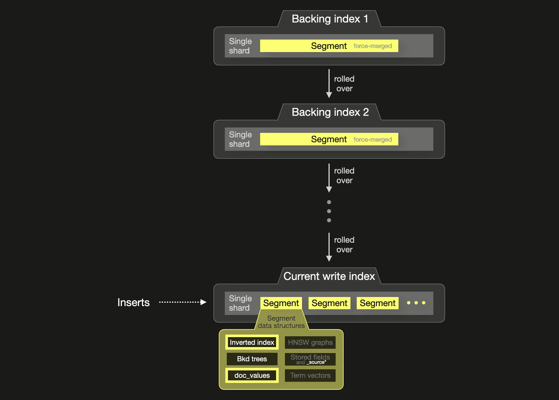
We used data streams for ingesting the data, where each data stream is backed by a sequence of automatically rolled over indices.
Since version 8.5, Elasticsearch also supports specialized time series data streams for timestamped metrics data. Comparing performance for metrics use cases is left for a future blog.
ILM policy
For the rollover thresholds, we used an index lifecycle management policy configuring the recommended best practices for optimal shard sizes (up to 200M documents per shard or a shard size between 10GB and 50GB). Additionally, to improve search speed and free up disk space, we configured that segments of a rolled-over index are force merged into a single segment.
Index settings
Number of shards
We configured the data stream’s backing indexes to consist of 1 primary and 0 replica shards. As described here, Elasticsearch uses one parallel query processing thread per shard for terms aggregations (which we use in our queries). Therefore, for optimal search performance, the number of shards should ideally match the number of 32 CPU cores available on our test machine. However, given the large ingested data amounts (billions of rows), the data stream’s automatic index rollovers will already create many shards. Furthermore, this is also a more realistic setup for a real-time streaming scenario (the original PyPi dataset is constantly growing).
Index codec
We tested storage sizes optionally with the heavier best_compression, which uses the DEFLATE instead of the default LZ4 codec.
Index sorting
To support an optimal compression ratio for the index codec and compact and access-efficient encoding of doc-ids for doc_values, we enabled index sorting and used all existing indexed fields for sorting stored fields (especially _source) and doc_values on disk. We listed the index sorting fields by their cardinality in ascending order (this ensures the highest possible compression rate).
Index mappings
We used component templates to create the PyPi data streams for Elasticsearch. The following diagram sketches a PyPi data stream:
The inserted documents contain 4 fields that we store in the index:
country_codeprojecturltimestamp
For a fair storage and performance comparison with ClickHouse, we switched off all segment data structures except inverted index, doc_values, and Bkd trees** for these fields by utilizing only the keyword and date data types in our index mappings. These aforementioned 3 data structures are relevant for data analytics access patterns like aggregations and sorts.
The keyword type populates the inverted index (to enable fast filtering) and doc_values (for aggregations and sorting). Additionally, for the inverted index the keyword type implies that there is no normalization and tokenization of the field values. Instead, they are inserted unmodified into the inverted index to support exact match filtering.
With this, the Elasticsearch inverted index (a lexicographically sorted list of all unique tokens pointing to document ID lists, with binary search lookups) becomes the approximate equivalent of the ClickHouse primary index (sparse lexicographically sorted list of primary key column values pointing to row blocks, with binary search lookups).
We could have further optimized the Elasticsearch data storage by disabling the inverted index for all fields (e.g. project and url) that our benchmark queries don’t filter on. This is possible by setting the index parameter for the keyword type to false in the index mapping. However, because these fields (project and url) are also part of our ClickHouse table’s primary key (and therefore, the ClickHouse primary index data structure is populated with values from these fields), we also kept the Elasticsearch inverted index for these fields.
The date type is internally stored as a long number in both doc_values (to support aggregations and sorting) and Bkd trees (queries on dates are internally converted to range queries utilizing Bkd trees). Because we use the date column also as a primary key column in ClickHouse, we didn’t switch off Bkd trees for the date field in Elasticsearch.
**In this blog, we focus on comparing the aggregation performance of the column-oriented
doc_valuesdata structure with ClickHouse’s columnar storage format and leave comparisons of other data structures for future blogs.
_source
To compare storage implications of _source, we used two different index mappings:
- one that stores
_source(see the segment data structure internals) - one that doesn’t store
_source
Note that by disabling _source, we reduce the data storage size. However, reindex (index to index copy) operations (e.g. for changing an index mapping in hindsight or to upgrade an index to a new major version) and update operations are no longer possible. Some queries also suffer with respect to performance because _source is the fastest way to retrieve field values in scenarios where all or a large subset of the indexed document fields are requested. Despite its much lower storage requirements, ClickHouse always allows table-to-table copy and update operations.
Transforms
For continuous data transformation, we created transforms for pre-calculating aggregations.
We optimized the automatically deduced index mappings for the transformed destination indexes to eliminate _source.
ClickHouse setup
Configuring ClickHouse is much simpler compared to Elasticsearch and requires less upfront planning and setup code.
ClickHouse configuration
ClickHouse is deployed as a native binary. We installed ClickHouse version 24.4 with default settings. No memory settings need to be configured. The ClickHouse server process needs about 1 GB of RAM plus the peak memory usage of executed queries. Like Elasticsearch, ClickHouse will utilize the rest of the machine’s available memory for caching data loaded from disk in the OS-level filesystem cache.
Tables
We created tables storing different sizes of the PyPi dataset with different compression codecs.
Column compression codec
Similar to Elasticsearch, we tested storage sizes optionally with the heavier ZSTD instead of the default LZ4 column compression codec.
Table sorting
For a fair storage comparison, we use the same data sorting scheme as in Elasticsearch to support an optimal compression ratio for the column compression codec. For this, we added all of the table’s columns to the table’s primary key, ordered by cardinality in ascending order (as this ensures the highest possible compression rate).
Table schema
The following diagram sketches a PyPi ClickHouse table:

Because ClickHouse runs on a single machine, each table consists, by default, of a single shard. Inserts create parts that are merged in the background.
The inserted rows contain exactly the same 4 fields as in the documents ingested into Elasticsearch. We store these in 4 columns in our ClickHouse table:
country_codeprojecturltimestamp
Based on our table schema, column data files are created for all 4 of our table’s columns. A sparse primary index file is created and populated from the values of the table’s sorting key columns. All other part data structures have to be explicitly configured and are not utilized by our benchmark queries.
Note that we use the LowCardinality type for the country_code column to dictionary-encode its string values. While this is a best practice for low cardinality columns in ClickHouse, it is not the primary reason for ClickHouse’s much lower storage requirements in this benchmark. In this case, with the PyPi data set, the storage saving is negligible compared to using the full String type for the country_code column, as the column’s low cardinality values are just 2-letter codes that compress well when the data is sorted by country_code.
Materialized views
For continuous data transformation, we created materialized views equivalent to the created Elasticsearch transforms for pre-calculating aggregations.
ClickHouse Cloud setup
As a side experiment, we run the same benchmark also on ClickHouse Cloud.
For this, we created the same aforementioned tables and materialized views and loaded the same data amount into a ClickHouse Cloud service featuring approximately the same hardware specifications as our EC2 test machines: 30 CPU cores and 120 GB RAM per compute node is the closest match. Note that ClickHouse uses a 1:4 CPU to Memory ratio. Furthermore, storage and compute are separated. All horizontally and vertically scalable ClickHouse compute nodes have access to the same physical data stored in object storage and are effectively multiple replicas of a single limitless shard:
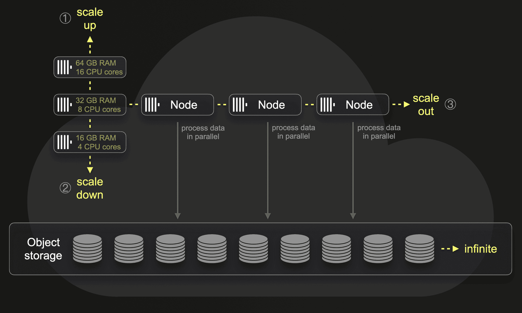
By default, each ClickHouse Cloud service features three compute nodes. Incoming queries are routed via a load balancer to one specific node that runs the query. It is straightforward to (manually or automatically) scale the size or number of compute nodes. Per parallel replicas setting, it is possible to process a single query in parallel by multiple nodes. This doesn’t require any physical resharding or rebalancing of the actual data.
We will run some of our benchmark queries with both a single node and multiple numbers of parallel nodes in our ClickHouse Cloud service.
Benchmark queries
The equivalent to a ClickHouse count(*) aggregation (using a SQL GROUP BY clause with a count(*) aggregate function) in Elasticsearch is the terms aggregation. We describe how Elasticsearch and ClickHouse process such queries under the hood here.
We test the (cold run) performance of the following count(*) aggregation queries on the raw (not pre-aggregated) data sets:
-
Query ① - Top 3 most popular PyPi projects: this is a full data scan aggregating the whole data set, sorting the aggregated data, and returning the top 3 buckets/groups
-
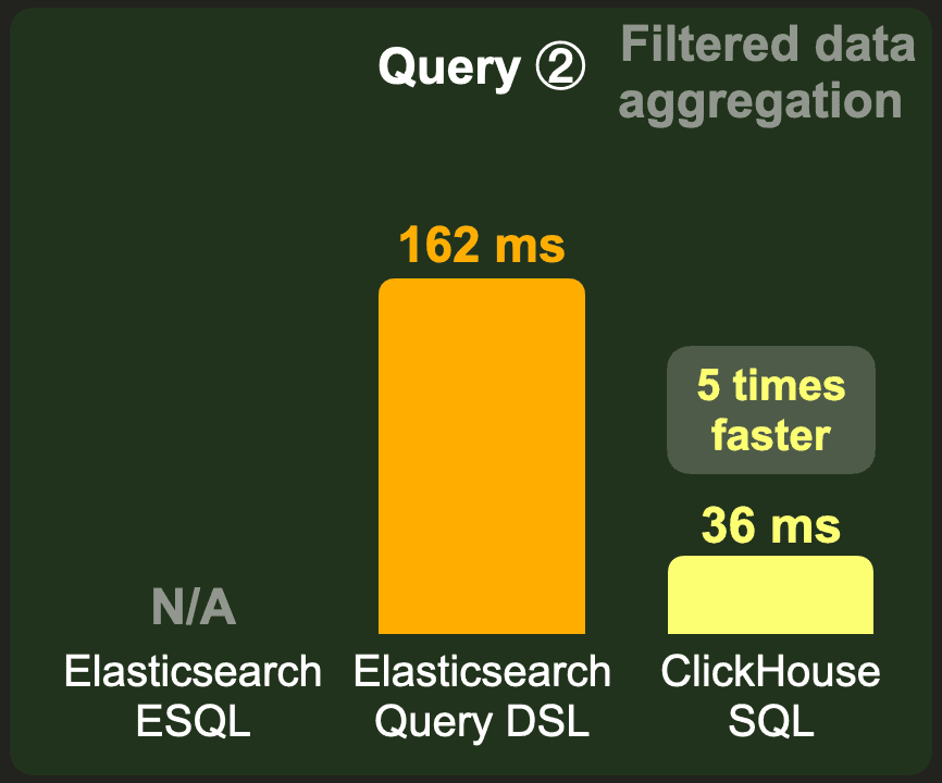
Query ② - Top 3 PyPi projects for a specific country: this query filters the data set before applying aggregation, sorting, and a limit.
We further test the performance of the same queries from above when they run over pre-aggregated data sets:
- Query ①
- ClickHouse SQL query
- Elasticsearch DSL query**
Elasticsearch ESQL query** (unsupported)
- Query ②
- ClickHouse SQL query
- Elasticsearch DSL query**
Elasticsearch ESQL query** (unsupported)
Note that for Elasticsearch we didn’t increase the term aggregation’s shard size parameter value in our benchmark.
**We noticed a slight issue when using Elasticsearch transforms for pre-calculating bucket sizes. For example, to pre-calculate the count per project. The way to do that is to group by project and then use a terms aggregation (also on project) to pre-calculate the count per project. The corresponding documents ingested into the destination index by the transform look like this:
{
"project_group": "boto3",
"project": {
"terms": {
"boto3": 28202786
}
}
}The transforms destination index mapping is this:
{
"project_group": {
"type": "keyword"
},
"project": {
"properties": {
"terms": {
"type": "flattened"
}
}
}
}Note the use of the flattened field type. It makes sense to use this type for the result values of the terms aggregation. Otherwise, each unique project name would need its own mapping entry, which is impossible to do upfront (we don’t know which projects exist) and would lead to a mapping explosion with dynamic mapping.
This creates two issues for our benchmark queries:
-
The flattened type is currently unsupported by ESQL.
-
All values are treated as keywords. When sorting, this implies that our numerical pre-calculated count values are compared lexicographically instead of in numerical order. Therefore, the Elasticsearch query running over indexes for transforms needs to use a small painless script to enable numerical sorting on the pre-calculated count values.
Benchmark methodology
With enabled caches, especially query result caches, both Elasticsearch and ClickHouse serve results almost instantaneously by just fetching them from a cache. We are interested in running aggregation queries with cold caches, where the query processing engine must load and scan the data and calculate the aggregation result from scratch.
Query Runtimes
We run all benchmark queries over the data sets that:
- Are compressed with the Elasticsearch and ClickHouse standard
LZ4codec - Don’t store
_sourcein Elasticsearch
All queries are executed three times with cold caches. We execute one query at a time i.e., measure latency only. In our charts in this blog, we take the average execution time as the final result and link to the detailed benchmark run results.
Elasticsearch
We run Elasticsearch queries (DSL) via the Search REST API and use the JSON response body’s took time, representing the total server-side execution time.
ESQL queries are executed with the ESQL REST API. Responses of Elasticsearch ESQL queries don’t include any runtime information. Server-side execution times for ESQL queries are logged in Elasticsearch’s log file, though.
We know that query runtimes are also available in the search slow log, but only on a per-shard level and not in consolidated form for the complete query execution over all involved shards.
ClickHouse
All ClickHouse SQL queries are executed via ClickHouse client, and the server-side execution time is taken from the query_log system table (from the query_duration_ms field).
Disabling caches
Elasticsearch
For query processing, Elasticsearch leverages the operating-system-level filesystem cache, the shard-level request cache, and the segment-level query cache.
For DSL queries, we disabled the request cache on a per-request basis with the request_cache-query-string parameter. For ESQL queries, this is not possible, though.
The query cache can only be enabled or disabled per index, but not per request. Instead, we manually dropped the request and query caches via the clear cache API before each query run.
There is no Elasticsearch API or setting for dropping or ignoring the filesystem cache, so we drop it manually using a simple process.
ClickHouse
Like Elasticsearch, ClickHouse utilizes the OS filesystem cache and a query cache for query processing.
Both caches can be manually dropped with a SYSTEM DROP CACHE statement.
We disabled both caches per query with the query’s SETTINGS clause:
… SETTINGS enable_filesystem_cache=0, use_query_cache=0;
Query peak memory usages
ClickHouse
We use the ClickHouse query_log system table to track and report queries' peak memory consumption (memory_usage field). As a bonus, we also report the data processing throughput (rows/s and GB/s) for some queries, as reported by the ClickHouse client. This can also be calculated from query_log fields (e.g. read_rows and read_bytes divided by query_duration_ms).
Elasticsearch
Elasticsearch runs all queries within the Java JVM, with half of the machine's available 64 GB RAM allocated at startup. Elasticsearch doesn’t directly track queries' peak memory consumptions within the JVM memory. The search profiling API, used under the hood of Kibana’s graphical search profiler, only profiles queries' CPU usage. Likewise, the search slow log only tracks runtimes but not memory. The Cluster stats API returns cluster and node-level metrics and statistics like current peak JVM memory usage, e.g. returned by this call:
GET /_nodes/stats?filter_path=nodes.*.jvm.mem.pools.old. It can be tricky to correlate these statistics with a specific query run as these are node-level metrics that consider all queries and wider processes, including background segment merges which can be memory intensive. Therefore, our benchmark results don’t report peak memory usage for the Elasticsearch queries.
Benchmark results
Summary
Before we present the benchmark results in full detail, we provide a brief summary.
1 billion rows data sets
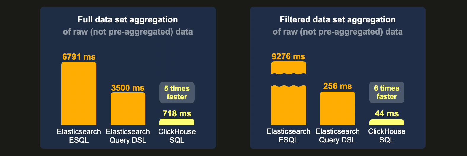
ClickHouse requires 12 times less disk space than Elasticsearch to store the 1 billion row data set on disk. Aggregation query ① (performing a full data set aggregation) runs 5 times faster over the raw (not pre-aggregated) data with ClickHouse than with Elasticsearch (Query DSL). Aggregation query ② (aggregating the filtered data set) runs 6 times faster with ClickHouse than with Elasticsearch (Query DSL).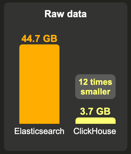
10 billion rows data sets
ClickHouse can store the raw data 19 times smaller than Elasticsearch and aggregate the full data set 5 times, and the filtered data set 7 faster.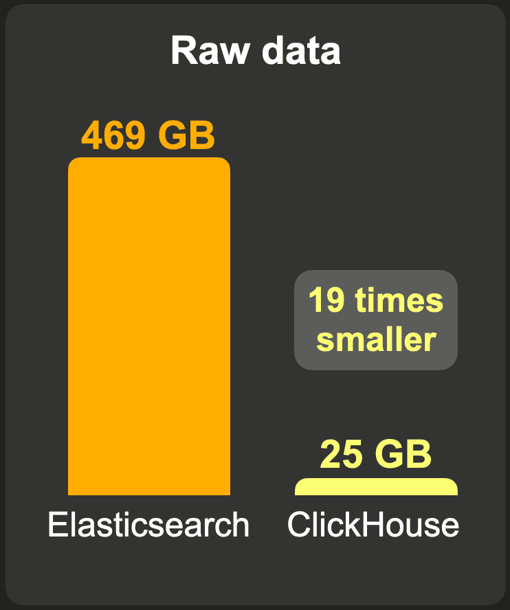
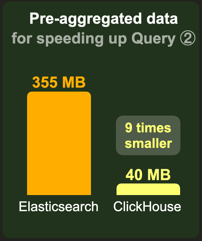
ClickHouse stores the data 7 times smaller and filters and aggregates it 5 times faster than Elasticsearch when the raw data is pre-aggregated to support speeding up aggregation query ②.
In the remainder of this section, we will first present in full detail the storage sizes for the PyPi data sets in raw (not pre-aggregated) and pre-aggregated form. After that, we will show detailed runtimes for running our aggregation queries over those data sets.
Storage size
Raw data
The following presents the storage sizes for the raw (not pre-aggregated) 1, 10, and 100 billion row PyPi data sets.
1 billion rows
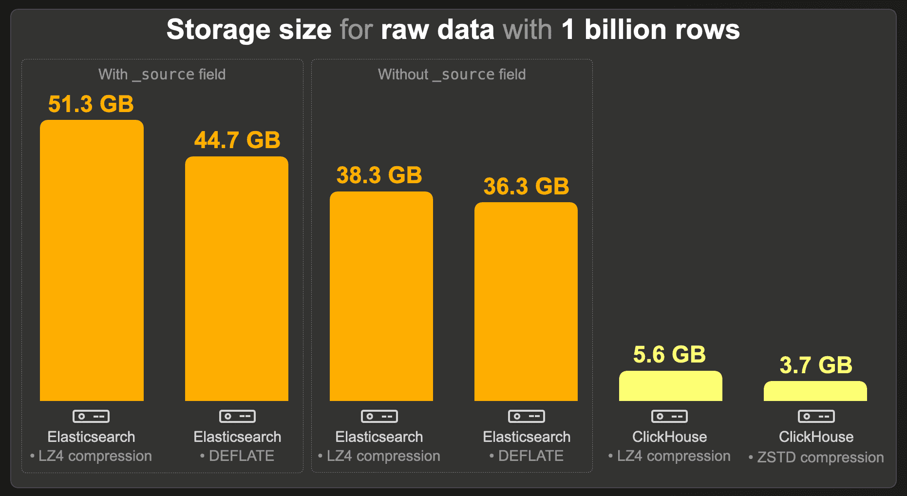
When _source is enabled, Elasticsearch requires 51.3 GB with its default LZ4 compression. With DEFLATE compression, this is reduced to 44.7 GB. As expected, our index sorting configuration enabled a high compression ratio for the index codecs: without index sorting, the index size would be 135.6 GB with LZ4 and 91.5 GB with DEFLATE.
Disabling _source reduced the storage to a size between 38.3 GB (LZ4) and 36.3 (DEFLATE).
The index codec (
LZ4orDEFLATE) is only applied tostored fields(which include_source) but not todoc_values, which is the main data structure remaining in our index with_sourcedisabled. And withindoc_values, each column is encoded individually (without usingLZ4orDEFLATE) based on data types and cardinality. Index sorting does support better prefix-compression fordoc_values, though, and enables a compact and access-efficient doc-ids encoding. But generally, the compression rate ofdoc_valuesdoesn’t benefit as much from index sorting asstored fields, e.g. without index sorting and withoutstored fields(disabled_source), the storage size of the Elasticsearch indexes is 37.7 GB (LZ4) and 35.4 (DEFLATE). (The fact that these sizes are even slightly smaller than those with index sorting is related to slightly different rollover times, causing different data structure overheads for shards and segments.)
Compared to an Elasticsearch index without _source field and equivalent compression levels (LZ4 vs. LZ4 and DEFLATE vs. ZSTD), a ClickHouse table requires approximately 7 times less storage space with LZ4 and about 10 times less with ZSTD compression.
The
_sourcefield is required in Elasticsearch to be functionally equivalent to ClickHouse (e.g. to enableupdateoperations and to runreindexoperations, equivalent to ClickHouseINSERT INTO SELECTqueries). When the same compression level is used (LZ4 vs. LZ4andDEFLATE vs. ZSTD), ClickHouse requires 9 to 12 times less storage space.
10 billion rows
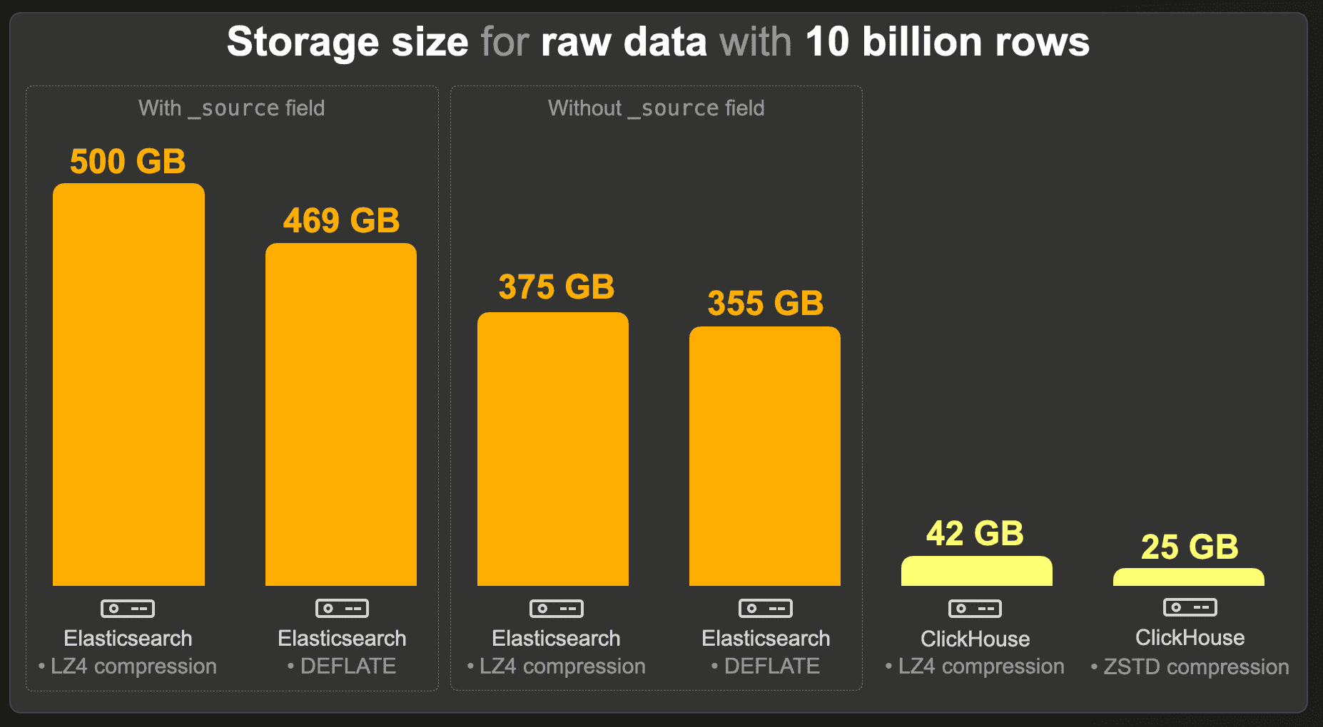
Like the 1 billion events data set, we measured storage sizes for Elasticsearch with and without _source and with default LZ4 and heavier DEFLATE codecs. Again, index sorting allows much better compression ratios (e.g. without index sorting, and with _source, the index size would be 1.3 TB with LZ4).
Compared to an Elasticsearch index without _source field and equivalent compression levels (LZ4 vs. LZ4 and DEFLATE vs. ZSTD), a ClickHouse table requires 9 times less storage than Elasticsearch and over 14 times less than Elasticsearch with ZSTD compression.
However, when Elasticsearch is functionally equivalent to ClickHouse (when we keep _source in Elasticsearch), and when the same compression level is used (LZ4 vs. LZ4 and DEFLATE vs. ZSTD), ClickHouse requires 12 to 19 times less storage space.
100 billion rows
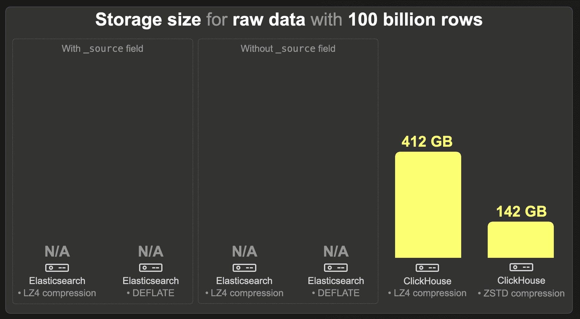
We were unable to load the 100 billion row data set into Elasticsearch.
ClickHouse requires 412 GB with LZ4 and 142 GB with ZSTD compression.
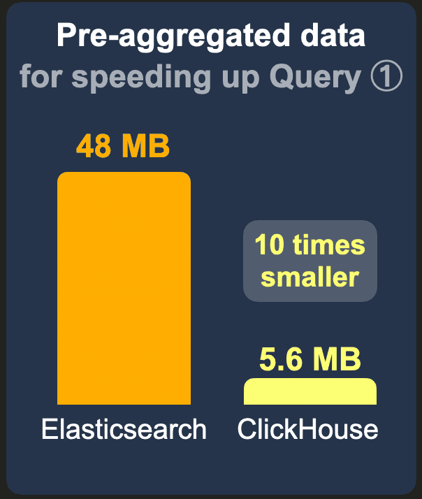
Pre-aggregated data for speeding up query ①
To significantly speed up our aggregation query ① calculating the top 3 most popular projects, we used transforms in Elasticsearch and materialized views in ClickHouse. These automatically converts the ingested raw (not pre-aggregated) data into separate pre-aggregated data sets. In this section, we present the storage sizes of those data sets.
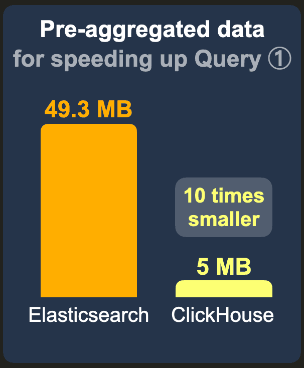
1 billion rows

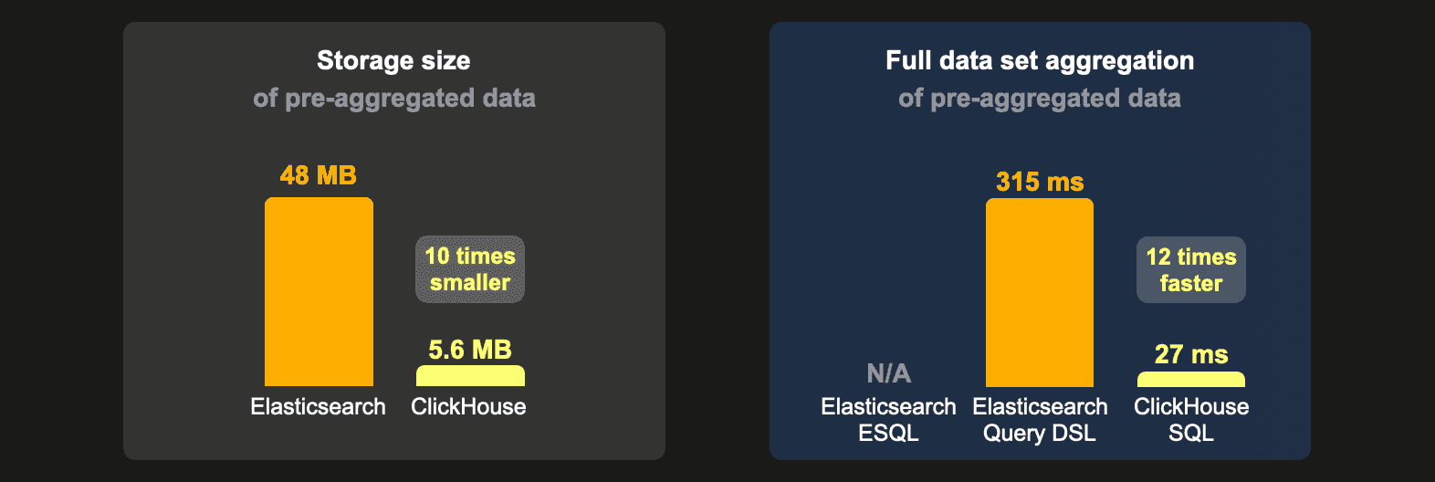
The data set with pre-aggregated counts per project contains only 434k instead of the raw 1 billion rows because there is 1 row with the pre-calculated count per 434k existing projects. We used the standard LZ4 compression codec for Elasticsearch and ClickHouse and disabled _source for Elasticsearch.
ClickHouse requires approximately 10 times less storage space than Elasticsearch.
10 billion rows
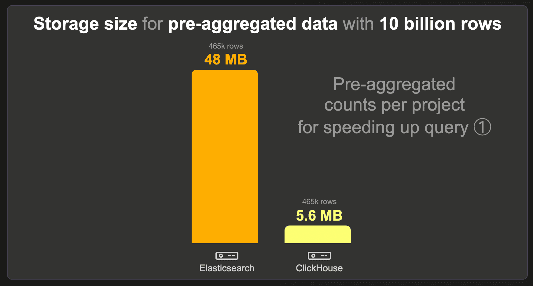
The data set with pre-aggregated counts per project contains only 465k instead of 10 billion rows because there is 1 row with the pre-calculated count per 465k existing projects. We used the standard LZ4 compression codec for Elasticsearch and ClickHouse and disabled _source for Elasticsearch.
ClickHouse requires over 8 times less storage space than Elasticsearch.
100 billion rows
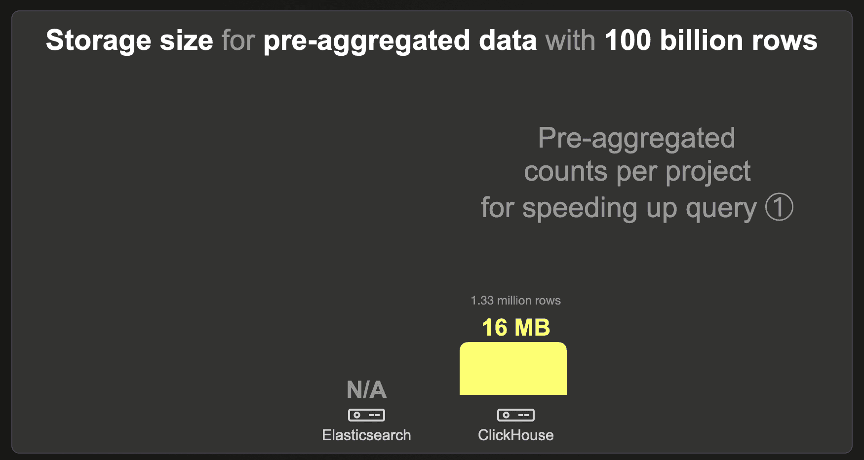
We were unable to load the 100 billion row data set into Elasticsearch.
ClickHouse requires 16 MB with LZ4 compression.
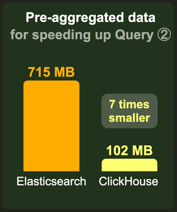
Pre-aggregated data for speeding up query ②
Also, for speeding up the Top 3 projects for a specific country aggregation query ②, we created separate pre-aggregated data sets, whose storage sizes we will list in the following.
1 billion rows
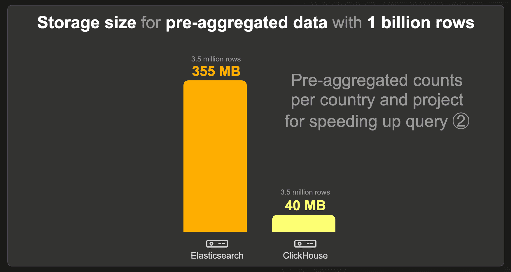
The data set with pre-aggregated counts per country and project contains 3.5 million instead of the raw 1 billion rows because there is 1 row with the pre-calculated count per existing country and project combination. We used the standard LZ4 compression codec for Elasticsearch and ClickHouse and disabled _source for Elasticsearch.
ClickHouse needs approximately 9 times less storage space than Elasticsearch.
10 billion rows
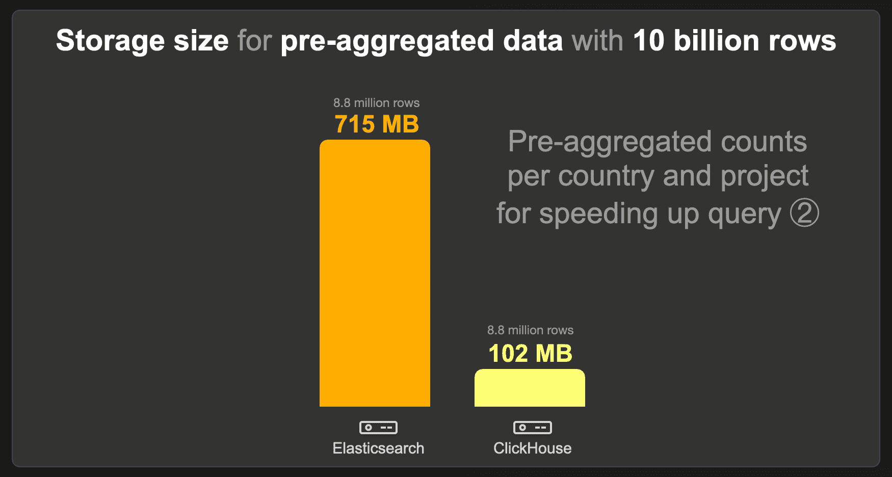
The data set with pre-aggregated counts per country and project contains 8.8 million instead of the raw 10 billion rows because there is 1 row with the pre-calculated count per existing country and project combination. We used the standard LZ4 compression codec for Elasticsearch and ClickHouse and disabled _source for Elasticsearch.
ClickHouse needs 7 times less storage space than Elasticsearch.
100 billion rows

We were unable to load the 100 billion row data set into Elasticsearch.
ClickHouse requires 480 MB with LZ4 compression.
Aggregation performance
This section presents the runtimes for running our aggregation benchmark queries over the raw (not pre-aggregated) and pre-aggregated data sets.
Query ① - Full data aggregation
This section presents the runtimes for our benchmark query ①, which aggregates and ranks the full data set.
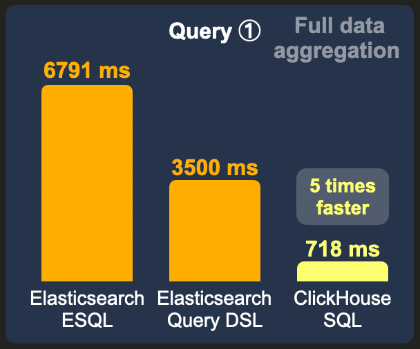
1 billion rows - Raw data
These are the cold query runtimes for running our top 3 most popular projects aggregation query over the raw (not pre-aggregated) 1 billion row data set:
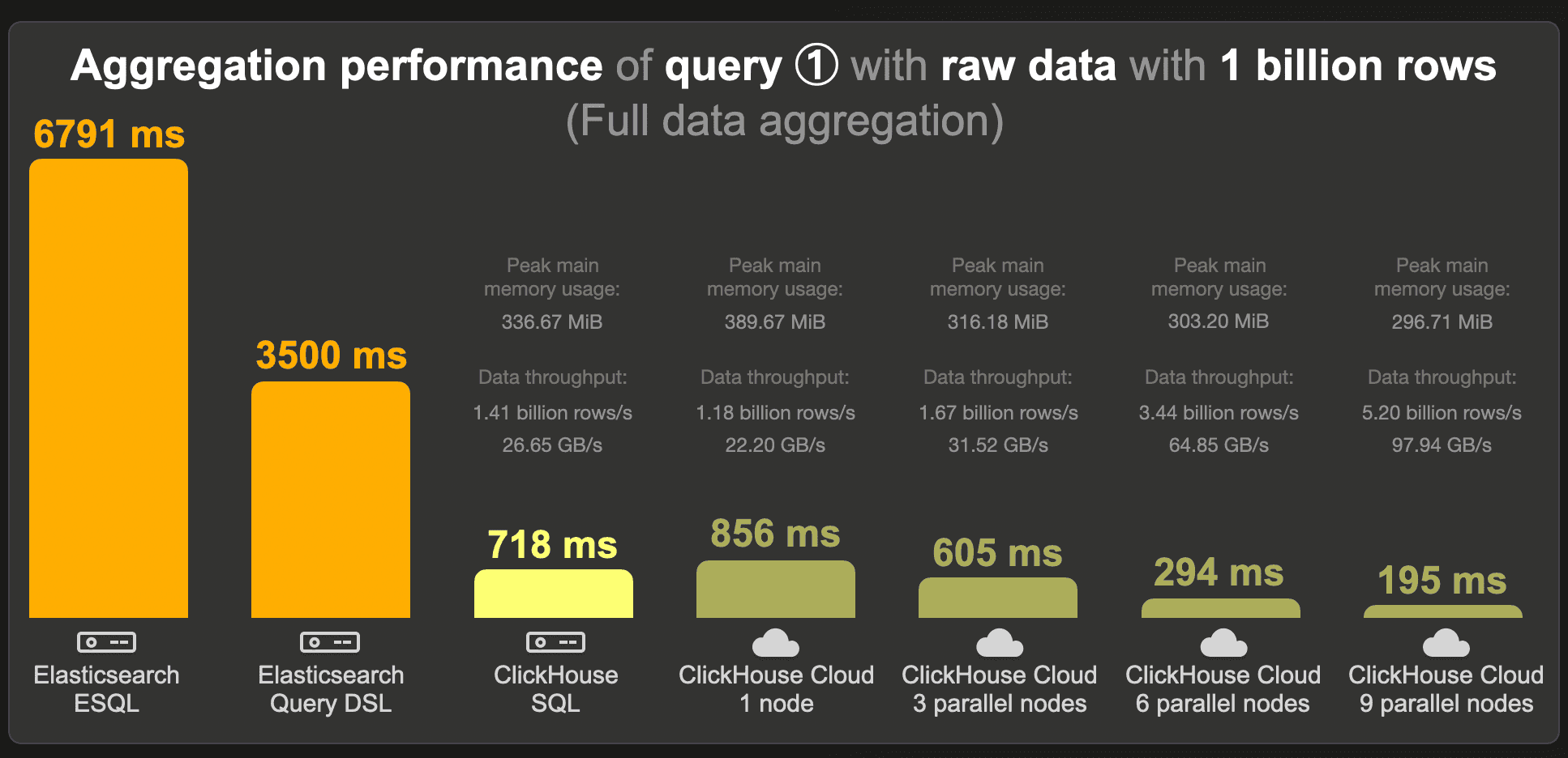
With its new ESQL query language, Elasticsearch runs the query in 6.8 seconds. Via traditional query DSL, the runtime is 3.5 seconds.
We noticed that on this dataset, query DSL seems to exploit the index sorting better than ESQL. When we optionally run the query over an unsorted index, the query DSL runtime is 9000 seconds, and ESQL is 9552 seconds.
ClickHouse runs the query approximately 5 times faster than Elasticsearch on the same machine size.
In ClickHouse Cloud, when running the query on a single (similarly sized) compute node, the cold runtime is a bit slower compared to open-source ClickHouse (as the data needs to be fetched from object storage into the node’s cache first). However, with node-parallel query processing enabled, a single 3-node ClickHouse Cloud service runs the query faster. This runtime can be further reduced by horizontal scaling. When running the query with 9 compute nodes in parallel, ClickHouse processes 5.2 billion rows per second with a data throughput of almost 100 GB per second.
Note that we annotated the ClickHouse runtimes with the query’s peak main memory usages, which are moderate for the amount of fully aggregated data.
We were curious to find the minimum machine size on which ClickHouse would run the aggregation query with a speed matching the Elasticsearch queries run on the 32-core EC2 machine. Or in other words, we are trying to see what smaller amount of resources would lead ClickHouse to be slower, and therefore more comparable, to Elasticsearch. The easiest and fastest way for this was downscaling the Elastic Cloud compute nodes, and running the query on a single node. With** 8 instead of 32 CPU cores**, the aggregation query runs in 2763 ms (cold runtime with disabled caches) on a single ClickHouse Cloud node. The 32 CPU core EC2 machine is a
c6a.8xlargeinstance with a price starting at $1.224 per hour. An 8 CPU cores instance would bec6a.2xlarge, whose price starts at $0.306 per hour, which is 4 times cheaper.
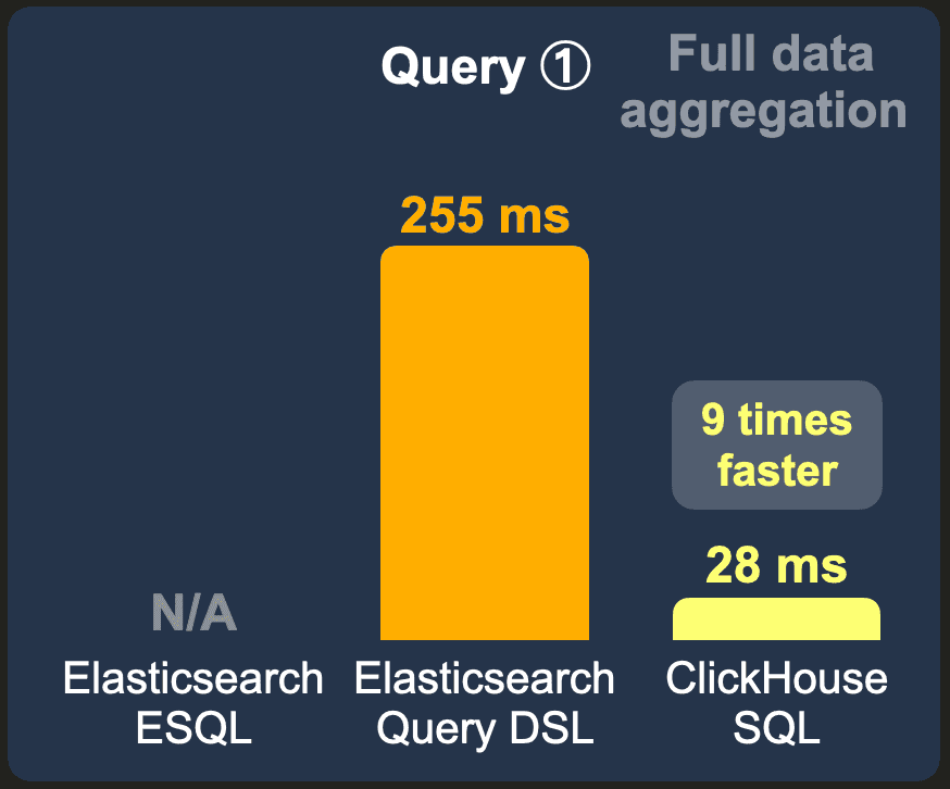
1 billion rows - Pre-aggregated data
These are the runtimes of running the top 3 most popular projects query over the data set with pre-aggregated counts instead of the raw 1 billion rows data set:
 As discussed, ESQL currently doesn’t support the flattened field type that is (needs to be) used in the Elastic transform generating the pre-aggregated data set.
ClickHouse runs the query 9 times faster than Elasticsearch, using ~ 75 MB of RAM. Again, because of low query latency, it doesn’t make sense to use parallel ClickHouse Cloud compute nodes for this query.
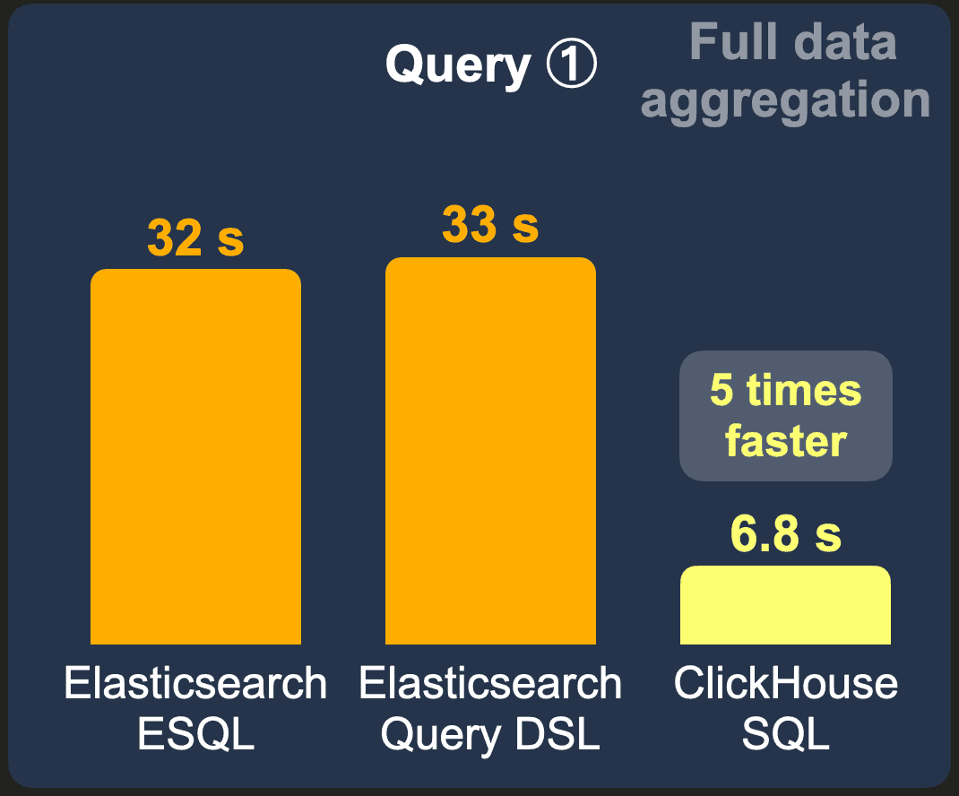
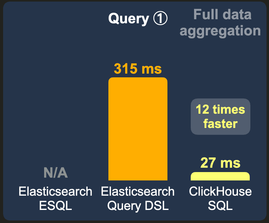
10 billion rows - Raw data
These are the cold query runtimes for running our top 3 most popular projects aggregation query over the raw (not pre-aggregated) 10 billion row data set:
 With an ESQL and a query DSL query, Elasticsearch needs 32 and 33 seconds, respectively.
ClickHouse runs the query approximately 5 times faster than Elasticsearch, using ~ 600 MB of RAM.
With 9 compute nodes in parallel, ClickHouse Cloud provides sub-second latency for aggregating the full 10 billion row data set, with a query processing throughput of 10.2 billion rows per second / 192 GB per second.
10 billion rows - Pre-aggregated data
These are the runtimes of running the top 3 most popular projects query over the data set with pre-aggregated counts instead of the raw 10 billion rows data set:
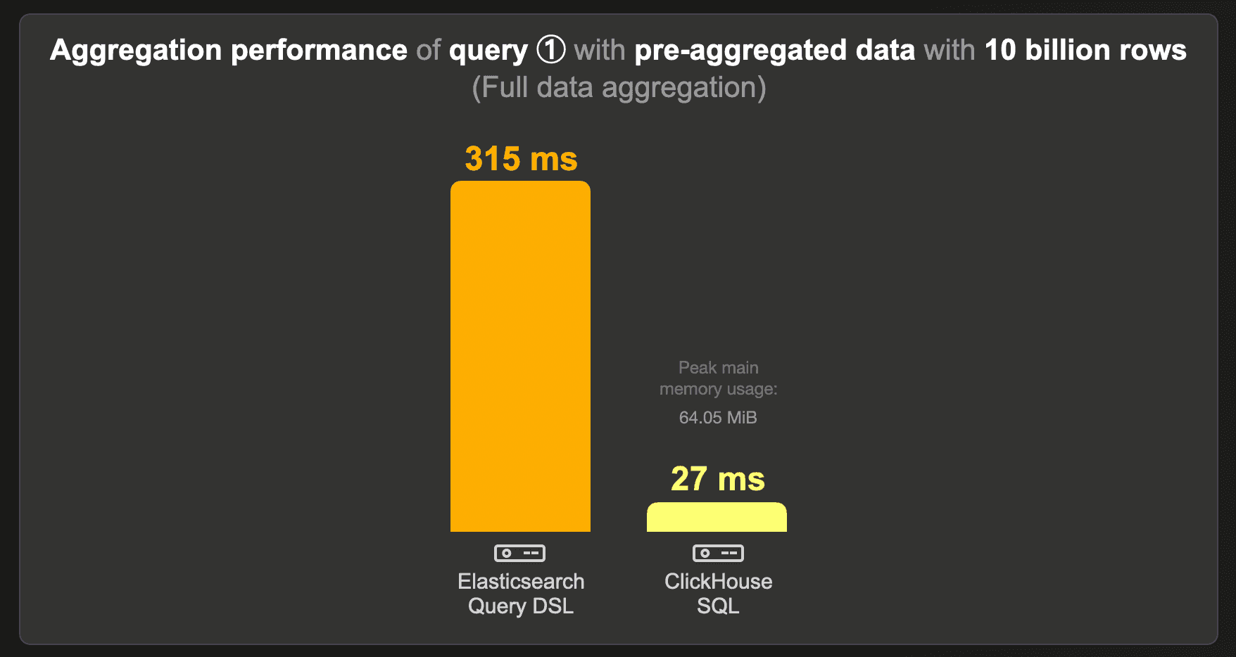
ClickHouse runs the query approximately 12 times faster than Elasticsearch, using ~ 67 MB of RAM.
100 billion rows - Raw data
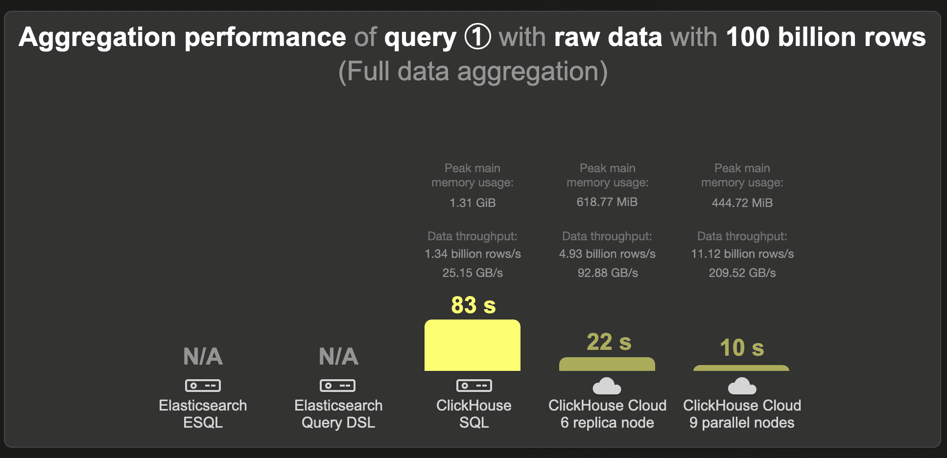
We were unable to load the 100 billion row data set into Elasticsearch.
We present the ClickHouse query runtimes here just for completeness. On our test machine, ClickHouse runs the query in 83 seconds.
100 billion rows - Pre-aggregated data
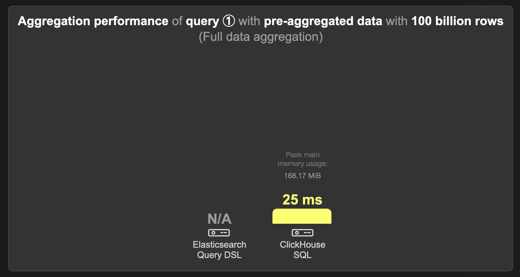
We were unable to load the 100 billion row data set into Elasticsearch.
ClickHouse runs the query in 25 ms.
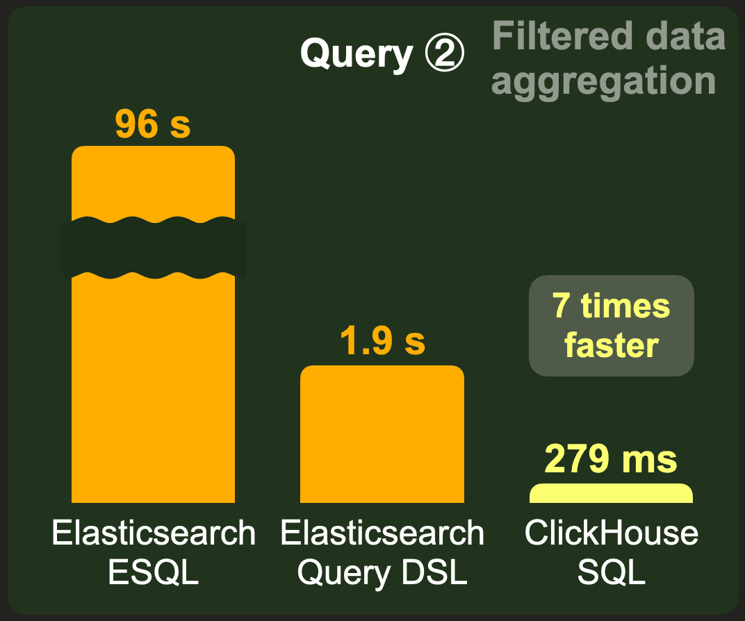
Query ② - Filtered data aggregation
This section shows the runtimes for our aggregation benchmark query ②, which filters the data set for a specific country before applying and ranking count(*) aggregations per project.
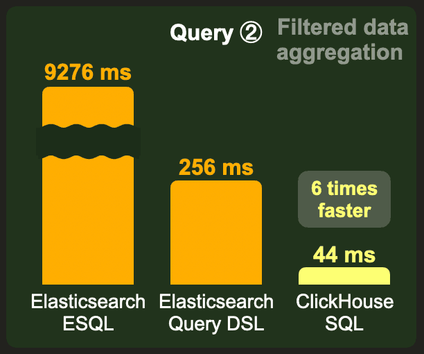
1 billion rows - Raw data
The following chart shows the cold runtimes for running the query that calculates the top 3 projects when the data set is filtered for a specific country over the raw (not pre-aggregated) 1 billion row data set:
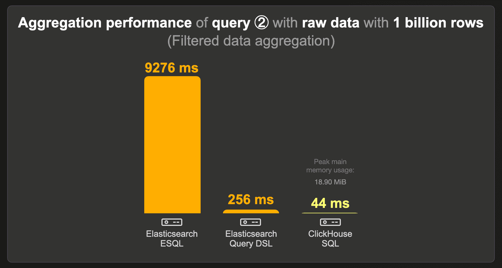
The Elasticsearch ESQL query has the highest runtime of 9.2 seconds. The equivalent query DSL variant runs significantly faster (256 ms).
ClickHouse runs this query approximately 6 times faster, and uses less than 20 MB of RAM.
Because of the low query latency, it doesn’t make sense to utilize parallel ClickHouse Cloud compute nodes for this query.
1 billion rows - Pre-aggregated data
These are the runtimes of running benchmark query ② (calculating the top 3 projects when the data set is filtered for a specific country) over the data set with pre-aggregated counts instead of the raw 1 billion rows data set:
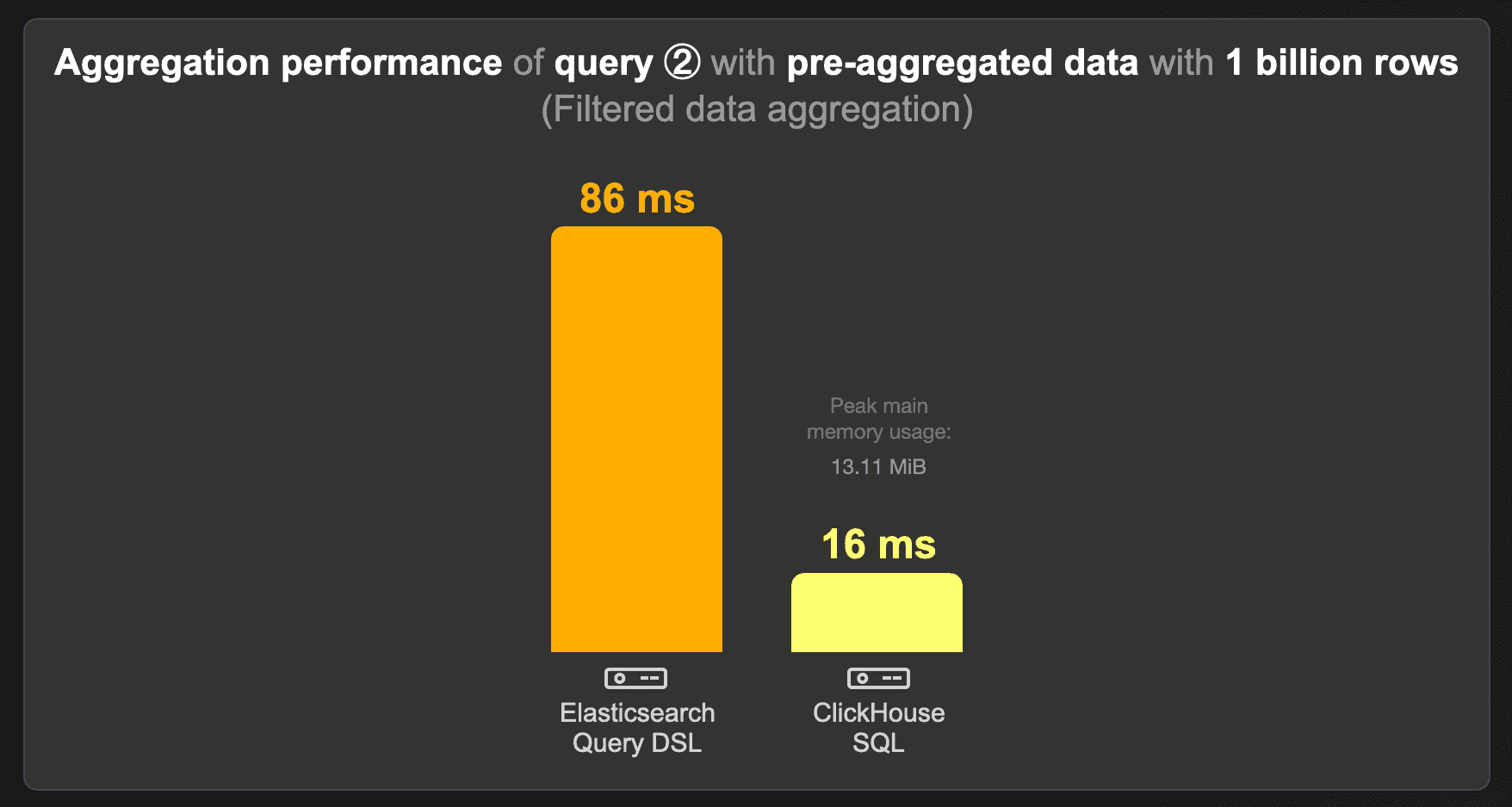
ClickHouse runs this query over 5 times faster than Elasticsearch, using ~ 14 MB of RAM.
10 billion rows - Raw data
This chart shows the cold runtimes for running benchmark query ② over the raw (not pre-aggregated) 10 billion row data set:
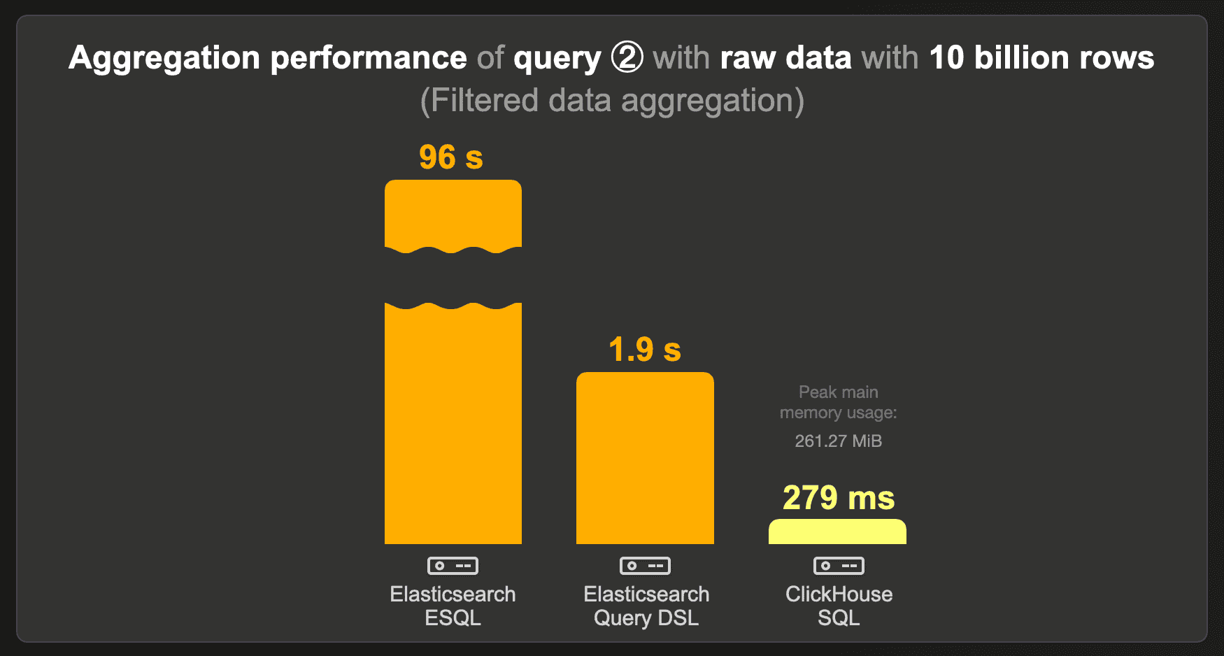
Elasticsearch ESQL doesn’t look good for this query, with a runtime of 96 seconds.
Compared to the Elasticsearch query DSL runtime, ClickHouse runs the query almost 7 times faster, consuming ~ 273 MB RAM.
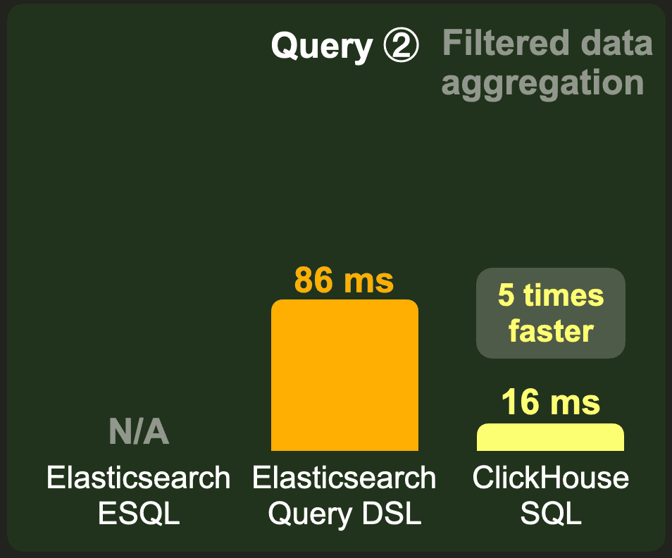
10 billion rows - Pre-aggregated data
These are the runtimes of running benchmark query ② over the data set with pre-aggregated counts instead of the raw 10 billion rows data set:
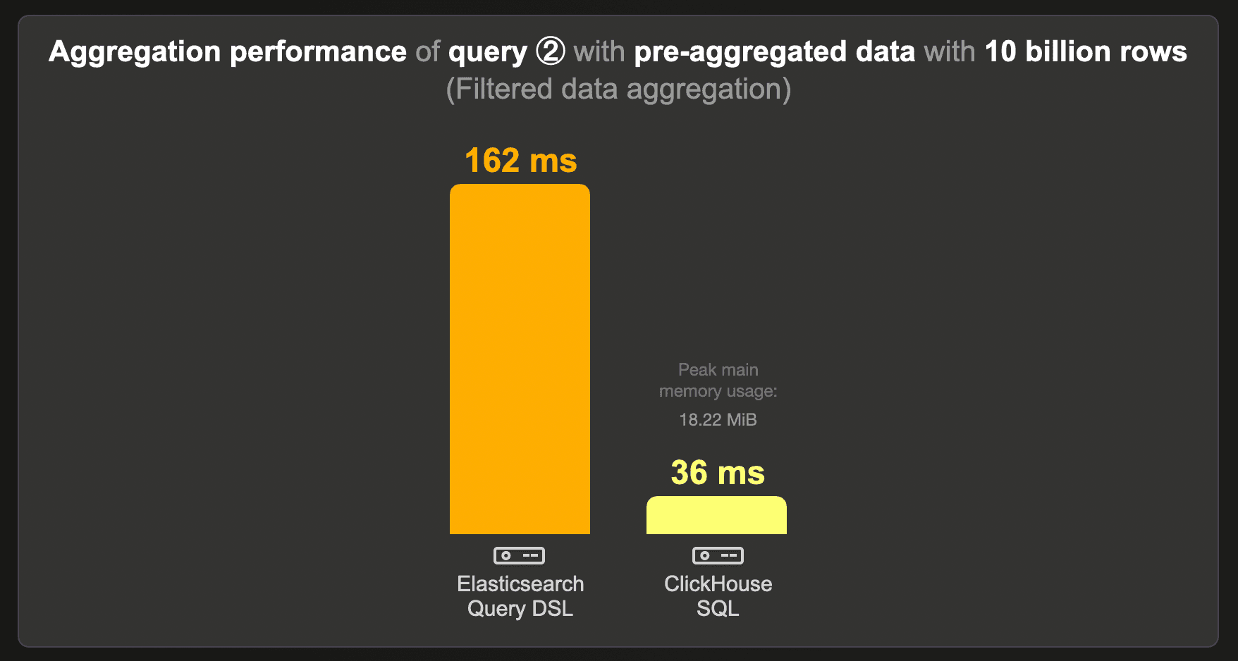
ClickHouse runs this query approximately 5 times faster than Elasticsearch, using ~ 19 MB of RAM.
100 billion rows - Raw data
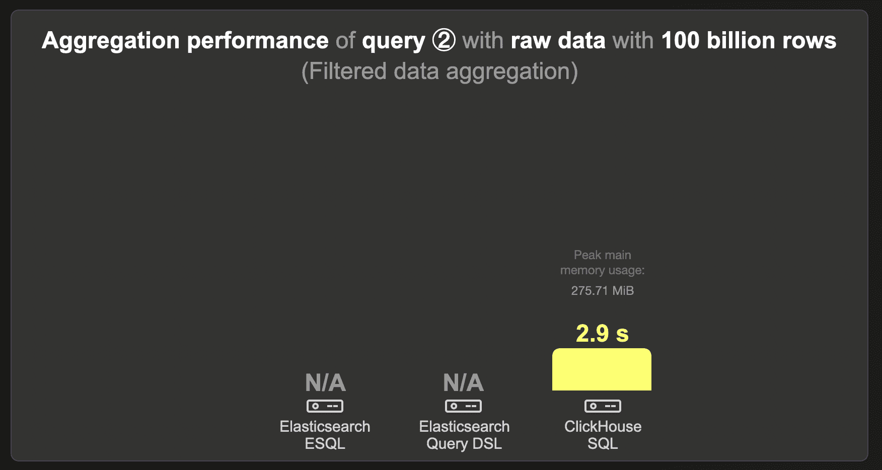
We were unable to load the 100 billion row data set into Elasticsearch.
ClickHouse runs the query in 2.9 seconds.
100 billion rows - Pre-aggregated data
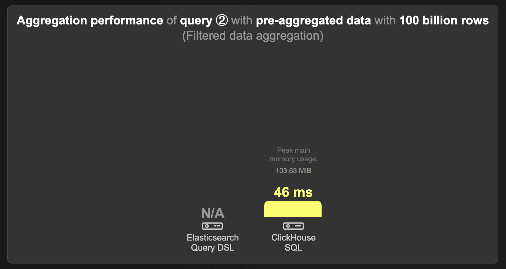
We were unable to load the 100 billion row data set into Elasticsearch.
ClickHouse runs the query in 46 ms.
Summary
Our benchmark demonstrated that for large data sets, typical in modern data analytics use cases, ClickHouse can store data more efficiently and run count(*) aggregation queries faster than Elasticsearch:
- ClickHouse requires 12 to 19 times less storage space, allowing smaller and cheaper hardware to be used.
- ClickHouse runs aggregation queries over raw (not pre-aggregated) and pre-aggregated data sets at least 5 times faster, requiring 4 times cheaper hardware for comparable Elasticsearch latencies.
- ClickHouse features a much more storage- and compute-efficient continuous data summarization technique, further lowering computing and storage costs.
Our accompanying blog post provides an in-depth technical explanation of why ClickHouse is so much faster and more efficient.
Potential follow-up pieces can compare multi-node cluster performance, query concurrency, ingestion performance, and metric use cases.
Stay tuned!


