Real-time tick data applications are a classic example of real-time analytics. Like tracking user behavior in web apps or monitoring metrics from IoT devices, they involve high-frequency event streams that need to be ingested, stored, and queried with low latency.
In financial markets, the difference is the urgency. Even a few seconds of delay can turn a profitable trade into a loss. Every trade and quote update generates a new tick, and these can number in the thousands per second across multiple symbols.
ClickHouse is a strong fit for this type of workload. It handles high-frequency inserts, time-based queries, and low latency queries. Built-in compression helps reduce storage overhead, even with billions of rows per symbol. Materialized views can be used to pre-aggregate or reorganize data as it's written, optimizing query performance without needing a separate processing layer.
In this post, we'll walk through how to build a real-time tick data application using Massive to access market data and ClickHouse to store and query ticks in real time. We'll put that together using NodeJS for the backend operation and React for the live visualization. Let's dive in.
What is a tick?
Before we begin, it helps to understand what a quote is and what a trade is. A quote represents the current prices at which market participants are willing to buy or sell a security. Specifically, it includes the best bid (the highest price someone is willing to pay) and the best ask (the lowest price someone is willing to sell for). These are continuously updated as new orders enter or exit the market.
| sym | bx | bp | bs | ax | ap | as | c | i | t | q | z | inserted_at |
|---|---|---|---|---|---|---|---|---|---|---|---|---|
| SPY | 12 | 602.73 | 2 | 11 | 602.74 | 6 | 1 | [1,93] | 1749583478206 | 63152225 | NYSE | 1749583479396 |
A trade, on the other hand, is an actual transaction between a buyer and a seller. It occurs when someone agrees to the current ask or bid price and an order is matched and executed. Trades are recorded with the executed price, the size of the trade, and a timestamp.
| sym | i | x | p | s | c | t | q | z | trfi | trft | inserted_at |
|---|---|---|---|---|---|---|---|---|---|---|---|
| SPY | 52983525034825 | 11 | 607.26 | 1 | [12,37] | 1750842255972 | 22126 | NYSE | 0 | 0 | 1750842257842 |
Tick data typically comes in two streams. One contains quote updates, and the other contains trade executions. Both are essential for understanding market behavior, but they serve different purposes in analysis and strategy development.
Access to real-time market data
Now we understand the type of data we're going to ingest, let's have a look at how to access it. We first need to find and subscribe to a stock market API. There are many available, the one we picked to build this demo is Massive. Their paid plan provides an unlimited call to their API, access to real-time data and support for Web sockets.
WebSockets are essential for streaming market data because they eliminate the latency and overhead of polling REST APIs. Instead of establishing new connections for each data request and potentially missing ticks between calls, WebSockets maintain a persistent connection that pushes data the moment it's available which is critical for high-frequency market data where milliseconds matter.
Starting to ingest data using Massive API is fairly straightforward, simply establish a connection with the /stocks endpoint, authenticate using your Massive API key and start processing messages.
Below is a code snippet implementation using NodeJS.
this.authMsg = JSON.stringify({
action: "auth",
params: process.env.MASSIVE_API_KEY,
});
this.ws = new WebSocket("wss://socket.polygon.io/stocks");
this.ws.on("open", () => {
console.log("WebSocket connected");
this.isConnected = true;
this.reconnectAttempts = 0;
this.lastMessageTime = Date.now();
this.connectionStartTime = Date.now();
this.statusMessage = "Connected - Authenticating...";
this.logConnectionEvent("connected");
this.ws.send(this.authMsg);
});
this.ws.on("message", (data) => {
if (!this.isPaused) {
this.handleMessage(data);
}
});Ingesting Data into ClickHouse
Modeling Tick Data in ClickHouse
Tick data is relatively straightforward to model since it consists of just two event types, one for trade and another one for quote, each with a small set of mostly numeric fields. Below is the DDL for creating two separate tables.
CREATE TABLE quotes
(
`sym` LowCardinality(String),
`bx` UInt8,
`bp` Float64,
`bs` UInt64,
`ax` UInt8,
`ap` Float64,
`as` UInt64,
`c` UInt8,
`i` Array(UInt8),
`t` UInt64,
`q` UInt64,
`z` Enum8('NYSE' = 1, 'AMEX' = 2, 'Nasdaq' = 3),
`inserted_at` UInt64 DEFAULT toUnixTimestamp64Milli(now64())
)
ORDER BY (sym, t - (t % 60000));
CREATE TABLE trades
(
`sym` LowCardinality(String),
`i` String,
`x` UInt8,
`p` Float64,
`s` UInt64,
`c` Array(UInt8),
`t` UInt64,
`q` UInt64,
`z` Enum8('NYSE' = 1, 'AMEX' = 2, 'Nasdaq' = 3),
`trfi` UInt64,
`trft` UInt64,
`inserted_at` UInt64 DEFAULT toUnixTimestamp64Milli(now64())
)
ORDER BY (sym, t - (t % 60000));The data volume can grow quickly.
For example, tracking trades on the Nasdaq alone can generate around 50 million records per day. Choosing an effective order key is essential for performance. In this case, rows are ordered first by sym (the stock symbol), grouping all events for the same symbol. Within each symbol group, rows are ordered by t - (t % 60000), which creates 1-minute time buckets. This approach works well in our case, as we aggregate data by symbol to generate the visualization. Grouping by minute improves the efficiency of time-based filtering and aggregation.
Ingestion strategy
There are several ways to design an ingestion pipeline for this type of application, including using a message queue like Kafka. However, to minimize latency, it's often better to keep the system simple and push data directly from the WebSocket connection into ClickHouse when possible.
Once that setup is in place, the next step is to choose the right ingestion method. ClickHouse supports both synchronous and asynchronous inserts.
With synchronous ingestion, data is batched on the client side before being sent. The batch size should strike a balance between memory usage, latency, and system overhead. Larger batches reduce the number of insert requests and improve throughput, but they can increase memory usage and delay individual records. Smaller batches reduce memory pressure but may create more load on ClickHouse by generating too many small data parts.
With asynchronous ingestion, data is sent to ClickHouse continuously, and batching is handled internally. Incoming records are first written to an in-memory buffer, which is then flushed to storage based on configurable thresholds. This method is useful when client-side batching isn't practical, such as when data comes from many small clients.
In our case, synchronous ingestion is a better fit. Since there's only one client pushing data from the WebSocket API, batching can be managed on the client side for better control over performance and resource usage.
Code snippet to ingest data from the NodeJS application.
handleMessage(data) {
try {
const trades = payload.filter((row) => row.ev === "T").map(({ ev, ...fields }) => fields);
const quotes = payload.filter((row) => row.ev === "Q").map(({ ev, ...fields }) => fields);
this.addToBatch(trades, "trades");
this.addToBatch(quotes, "quotes");
} catch (error) {
console.error("Error handling message:", error);
console.error("Message data:", data.toString().substring(0, 200));
}
addToBatch(rows, type) {
if (rows.length === 0) return;
const batch = type === "trades" ? this.tradesBatch : this.quotesBatch;
batch.push(...rows);
if (batch.length >= this.maxBatchSize) {
this.flushBatch(type);
}
}
flushBatch(type) {
const batch = type === "trades" ? this.tradesBatch : this.quotesBatch;
if (batch.length === 0) return;
const dataToInsert = [...batch];
if (type === "trades") {
this.tradesBatch = [];
} else {
this.quotesBatch = [];
}
await this.client.insert({
table: table,
values: data,
format: "JSONEachRow",
});
}Visualize live market data
Once the data is stored in ClickHouse, building the visualization layer is straightforward. The main challenge lies in writing the right SQL queries. Let’s have a look on how to achieve this. We’ll focus on the queries needed to power two key visualizations. The first is a real-time table that updates continuously to show the latest trading data for a specific stock.
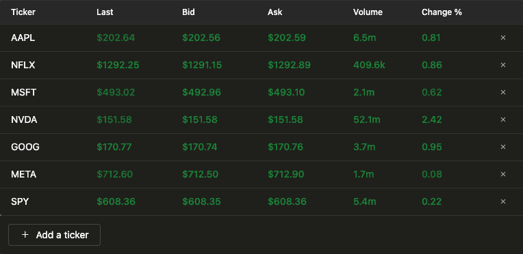
To build this visualization, one query is enough, the data can be formatted using ClickHouse's powerful SQL query language and custom functions.
WITH
{syms: Array(String)} as symbols,
toDate(now('America/New_York')) AS curr_day,
trades_info AS
(
SELECT
sym,
argMax(p, t) AS last_price,
round(((last_price - argMinIf(p, t, fromUnixTimestamp64Milli(t, 'America/New_York') >= curr_day)) / argMinIf(p, t, fromUnixTimestamp64Milli(t, 'America/New_York') >= curr_day)) * 100, 2) AS change_pct,
sum(s) AS total_volume,
max(t) AS latest_t
FROM trades
WHERE (toDate(fromUnixTimestamp64Milli(t, 'America/New_York')) = curr_day) AND (sym IN (symbols))
GROUP BY sym
ORDER BY sym ASC
),
quotes_info AS
(
SELECT
sym,
argMax(bp, t) AS bid,
argMax(ap, t) AS ask,
max(t) AS latest_t
FROM quotes
WHERE (toDate(fromUnixTimestamp64Milli(t, 'America/New_York')) = curr_day) AND (sym IN (symbols))
GROUP BY sym
ORDER BY sym ASC
)
SELECT
t.sym AS ticker,
t.last_price AS last,
q.bid AS bid,
q.ask AS ask,
t.change_pct AS change,
t.total_volume AS volume
FROM trades_info AS t
LEFT JOIN quotes_info AS q ON t.sym = q.sym;Let's break down what this query does.
First, it defines two variables: symbols, which holds the list of stock tickers to analyze, and curr_day, which captures the current date in the New York timezone.
The query then retrieves trade data, including:
last_price: The most recent trade price, usingargMax(p, t)to get the price at the latest timestampchange_pct: The percentage change from the day's opening price.total_volume: Total volume for the day
It also fetches quote data:
bid: Most recent bid price usingargMax(bp, t)ask: Most recent ask price usingargMax(ap, t)
Finally, the trade and quote results are joined to produce the final output.
| ticker | last | bid | ask | change | volume |
|---|---|---|---|---|---|
| NVDA | 151.2099 | 151.2 | 151.21 | 2.17 | 65269276 |
The second visualization we’re going to analyze is a candlestick visualization that shows the price evolution and volume for a given stock.
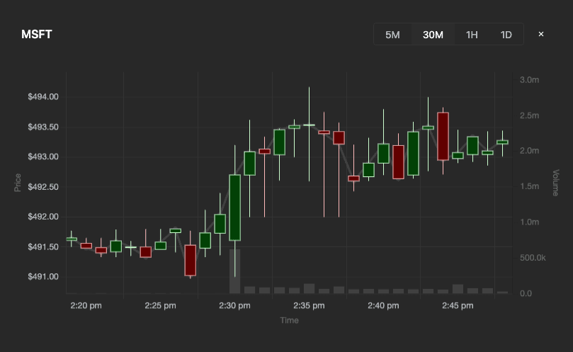
Let’s have a look at the SQL query to power this visualization.
SELECT
toUnixTimestamp64Milli(toDateTime64(toStartOfInterval(fromUnixTimestamp64Milli(t), interval 2 minute), 3)) as x,
argMin(p, t) as o,
max(p) as h,
min(p) as l,
argMax(p, t) as c,
sum(s) as v
FROM trades
WHERE x > toUnixTimestamp64Milli(now64() - interval 1 hour) AND sym = {sym: String}
GROUP BY x
ORDER BY x ASC;This query is simpler, as it only computes the trading volume, along with the highest and lowest prices, over a specified time window.
To visualize the query result, we use click-ui components for the table display and Chart.js for the candlestick visualization.
Scaling and practical tips
Handling high-frequency market data in production requires more than just a fast database. The following tips and techniques help ensure your system remains performant and reliable as data volume grows.
Scaling ingestion
When dealing with tick-level data across many symbols, sustained throughput can easily exceed tens of thousands of records per second.
To handle this there are different things to look for:
- Use client-side batching with insert sizes optimized for your system's memory and latency constraints.
- Use compression: Compressing insert data reduces the size of the payload sent over the network, minimizing bandwidth usage and accelerating transmission.
- Monitor the number of parts created in ClickHouse to prevent excessive merging. This blog talks about asynchronous insert, but the part creation section can be applied for a synchronous ingestion. You can also use advanced dashboards to monitor the number of data parts.
- Massive also provides performance tips to handle high volume data consumption.
Monitoring ingest latency
As discussed earlier, having the freshest data is critical for a financial application. So it does make sense to monitor it.
You can easily calculate and track the difference between the event timestamp (when the tick occurred) and the ingestion timestamp (when it was stored). This “ingest delay” is key to detecting backpressure or performance bottlenecks.
SELECT
sym,
count() AS trade_count,
argMax(inserted_at, t) - argMax(t, t) AS ingest_latency
FROM trades
GROUP BY sym
ORDER BY trade_count DESC
LIMIT 100;Visualizing this metric in a dashboard helps you catch slowdowns early.
Take advantage of materialized views
Materialized views are useful when you want to pre-aggregate data as it arrives. This helps optimize specific query patterns that rely on time-based summaries. A typical example is computing OHLCV (Open, High, Low, Close, Volume) metrics for financial data at fixed intervals, such as 1-minute windows. By generating these aggregates during ingestion, you can serve results quickly without recalculating them each time.
Start by creating a destination table to store the 1-minute OHLCV aggregates. This table will receive the output from the materialized view and provide a structured way to access precomputed results.
-- Create destination table
CREATE TABLE trades_1min_ohlcv
(
`sym` LowCardinality(String),
`z` Enum8('NYSE' = 1, 'AMEX' = 2, 'Nasdaq' = 3),
`minute_bucket_ms` UInt64,
`open_price_state` AggregateFunction(argMin, Float64, UInt64),
`high_price_state` AggregateFunction(max, Float64),
`low_price_state` AggregateFunction(min, Float64),
`close_price_state` AggregateFunction(argMax, Float64, UInt64),
`volume_state` AggregateFunction(sum, UInt64),
`trade_count_state` AggregateFunction(count)
)
ENGINE = SummingMergeTree
ORDER BY (sym, minute_bucket_ms);The next step is to create the materialized view.
-- Create view
CREATE MATERIALIZED VIEW trades_1min_ohlcv_mv TO trades_1min_ohlcv
AS SELECT
sym,
z,
intDiv(t, 60000) * 60000 AS minute_bucket_ms,
argMinState(p, t) AS open_price_state,
maxState(p) AS high_price_state,
minState(p) AS low_price_state,
argMaxState(p, t) AS close_price_state,
sumState(s) AS volume_state,
countState() AS trade_count_state
FROM trades
GROUP BY
sym,
z,
minute_bucket_ms;Now as each trade insert hits the trades table, the materialized view automatically processes it and updates the corresponding 1-minute bucket in the destination table.
To view the data, execute this query.
-- Query the table
SELECT
sym,
z,
minute_bucket_ms,
fromUnixTimestamp64Milli(minute_bucket_ms) as minute_timestamp,
argMinMerge(open_price_state) AS open_price,
maxMerge(high_price_state) AS high_price,
minMerge(low_price_state) AS low_price,
argMaxMerge(close_price_state) AS close_price,
sumMerge(volume_state) AS volume,
countMerge(trade_count_state) AS trade_count
FROM trades_1min_ohlcv
GROUP BY sym, z, minute_bucket_ms
ORDER BY sym, z, minute_bucket_ms;Conclusion
In this post, we explored how to build a real-time tick data application using Massive for market data and ClickHouse for fast ingestion and querying. We covered how to stream and structure tick data, manage ingestion performance, and build efficient queries and visualizations.
In this Github repository, you will find a working example of this using React for the visualization layer. While this is a simple example, the same principles would apply when building a production ready application at scale.


