You'll often hear us say that ClickHouse is not significantly affected by high cardinality when used for observability workloads. While directionally true, that statement only really makes sense once you understand why high cardinality becomes problematic in traditional time-series systems in the first place. This post is intended as background for a follow-on post exploring why high cardinality behaves differently in ClickHouse and other column-oriented databases. We’ll focus primarily on Prometheus, since it remains the dominant metrics store in observability and clearly illustrates the tradeoffs of a series-oriented storage model. We’ll show where cardinality costs appear: series creation, memory use, querying, and churn from short-lived infrastructure.
If you’re already familiar with high cardinality, Prometheus internals, series churn, and the operational challenges cardinality creates in time-series systems, you can likely skip ahead to Part 2, where we explore how ClickHouse handles these workloads differently.
What is high cardinality in Observability?
In observability systems, high cardinality usually means many unique label combinations.
We’ll use Prometheus as the reference model because it remains the dominant metrics store in observability. Additionally, although alternatives to it exist, they are typically built on the same fundamental data model.
Not all time series databases are implemented in the same way as Prometheus, and each has its own internal architecture and storage engine. However, many systems that model data as distinct time series, as described below, will face similar challenges when cardinality grows.
In time-series databases, cardinality refers to the number of unique label combinations. For this to make sense, we need to take a step back and define a metric, a label, and a time series.
To define what a label is, it's helpful to define what a metric is. A metric is effectively an observable numeric property e.g. "number of HTTP requests” or “current temperature". A metric can have extra dimensions known as labels. These string values effectively tell us what the metric is about, with each label having a value from a set.
A time series is an instance of a metric, with a unique combination of labels. It holds a series of timestamps and values.
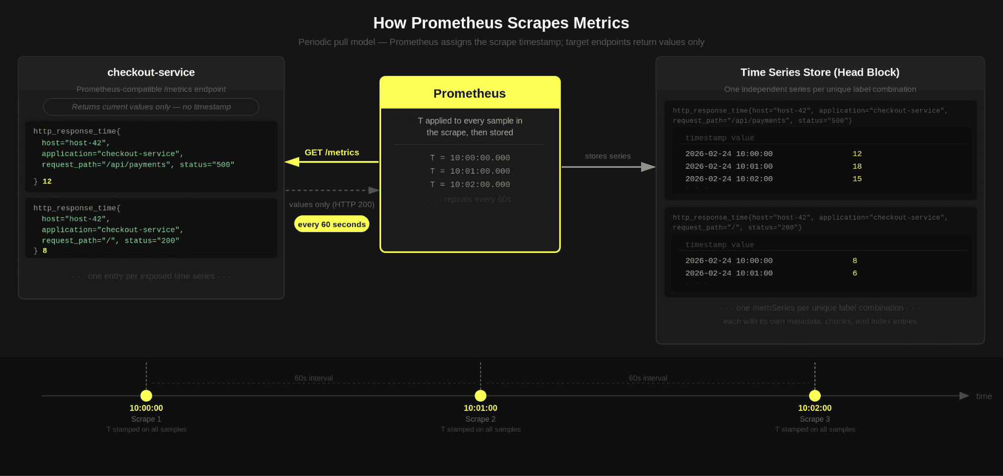
Suppose you have a gauge metric like http_response_time representing the most recent observed response time, with labels such as host, application, request_path, and status. A series might look like the following:
http_response_time {
host="host-42",
application="checkout-service",
request_path="/api/payments",
status="500"
}This series can have a set of timestamps and values e.g.
(2026-02-24 10:00:00, 12)
(2026-02-24 10:01:00, 18)
(2026-02-24 10:02:00, 15)
...Effectively, the labels tell us what's being observed, and the timestamp and values tell us how it changed over time. These timestamp+values can then be rendered as a series on a chart. A metric can therefore have one or more time series. The exact number depends on the number of unique label values.
Prometheus typically collects data by scraping a Prometheus-compatible HTTP endpoint that exposes the current value of each time series at the moment of the scrape (a sample), without an explicit timestamp. Prometheus assigns the scrape time as the timestamp for every sample it records. In effect, it periodically captures a snapshot of all exposed metrics and associates the scrape timestamp with each time series value returned during that interval.
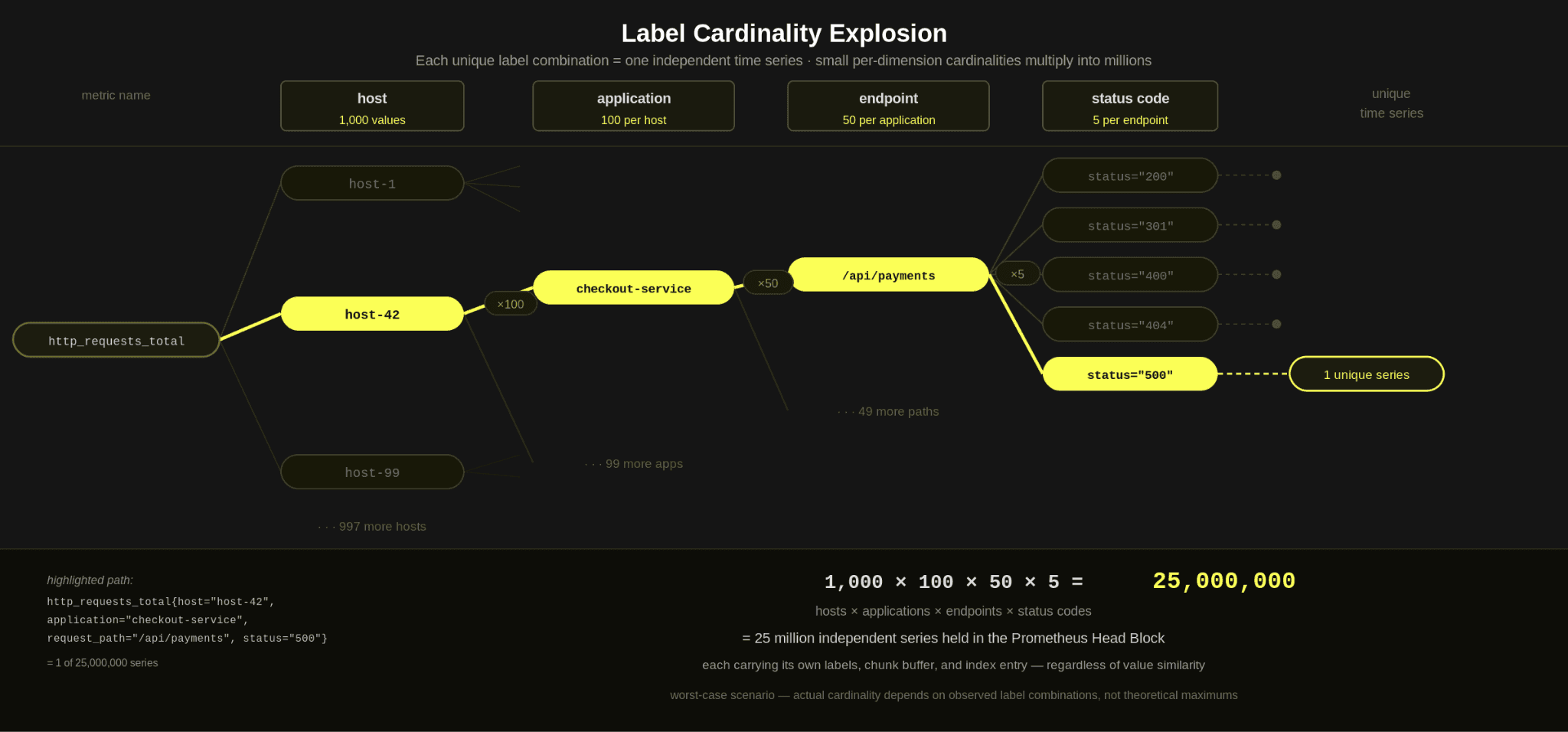
So, while a series looks simple individually, in totality, it introduces complexity. Cardinality is not just about one label having many unique values. It is about the total number of unique combinations across all labels i.e. the number of unique time series.
For example, consider the above http_requests_total metric - if host had a cardinality of 1000, application 100, endpoint 50, and the status code 5 - and we captured a metric for each unique value, we potentially have the following number of time series:
1,000 × 100 × 5 × 50 = 25,000,000 unique time series
This is obviously a worst-case scenario - it assumes that every application runs on every host and that the endpoints exist for each application. But it is before additional realistic dimensions are introduced, like region, environment, version, or container ID.
Cardinality is the number of unique time series, and high cardinality is when you have a lot of them!
Finally, it's worth noting that adding a single label to a metric can significantly increase the number of time series (up to the product of the new label's cardinality) due to the compounding problem.
Prometheus and the time series data model
Continuing with Prometheus as our example database, the fundamental unit of storage is the series itself. Every unique combination of labels for a metric creates a new series, and every series carries its own overhead. As we noted above, adding a label to a time series can significantly increase its cardinality.
But why is there such a significant overhead for each time series?
The answer lies in how the Prometheus server handles these series internally.
Data structures and memory overhead
When Prometheus scrapes a sample, it first needs to check if the series has been seen before. Series can be identified by their metric name and a unique set of label values. The label set and metric name are therefore hashed to produce a unique series identifier, and the series is looked up. This lookup is fast and predictable, effectively a hash table lookup over the in-memory series index.
Assuming the time series exists, the new sample needs to be appended to an existing in-memory structure - a memSeries. In addition to the label values, this holds all samples and their respective timestamps. This append operation is low-cost and represents the common hot path.

If the series doesn't exist, a memSeries needs to be created and registered with internal structures. This creation work happens on the write path, so it directly affects ingestion latency.
There is some important nuance in how samples in memSeries are managed as well. By default, Prometheus keeps up to two hours of recent data in memory in what is called the Head block. Within the Head, each active time series stores its samples in compressed chunks (rather than as individual points) that the memSeries references. These chunks are typically sized to hold 120 samples by default.
If a metric is scraped once per minute, that means a single chunk will span the two hours of data for each series in the head block. If samples are collected more frequently, chunks will fill faster, and additional chunks will be allocated within the same two-hour window. As a result, higher scrape frequencies increase the number of in-memory chunks per series, thereby increasing memory consumption.
The actual overhead for each series thus depends on a few factors:
- The memSeries struct and the fields it needs ~ 200 bytes itself
- The number and size of the labels
- The number of samples for each series and the resulting chunks. Note: Each chunk also has a metadata overhead.
In summary, two factors drive the memory usage of the head block: the number of series and the number of samples per series.
The decision to store each series independently means each series inherently incurs metadata overhead for itself, its labels, and its chunks.
Prometheus stores regular float samples using an XOR-based encoding where each value is stored as the XOR against the previous value, plus a compact “delta-of-deltas” encoding for timestamps. Both timestamp deltas and XOR values are packed using variable-width bit encodings. This compression technique is well-suited to long-lived time series data that are being scraped at set intervals and where the samples don’t change.
This is before we factor in additional system-wide structures, such as an inverted index, that enable queries to find series by label selectors. This inverted index effectively stores, for each label name and value, a list of references to all series that contain that label pair. As cardinality increases, these posting lists grow, adding further memory overhead and increasing the work required to evaluate queries that match across many label combinations.
Storing structures to disk
As described above, the Head block holds roughly two hours of recent data in memory. To prevent unbounded memory growth, Prometheus periodically cuts the Head into a persistent block on disk.
In practice, this occurs at roughly two-hour block boundaries, with recently written chunks remaining in the Head until truncation. At that point, the compressed chunks for this time range are written to disk as part of a new block.
Recent data lives in memory, and every couple of hours, it is sealed and persisted. Once written to disk, the in-memory chunk data for that time range can be released from the Head. The data is then retained on disk for the specified retention period.
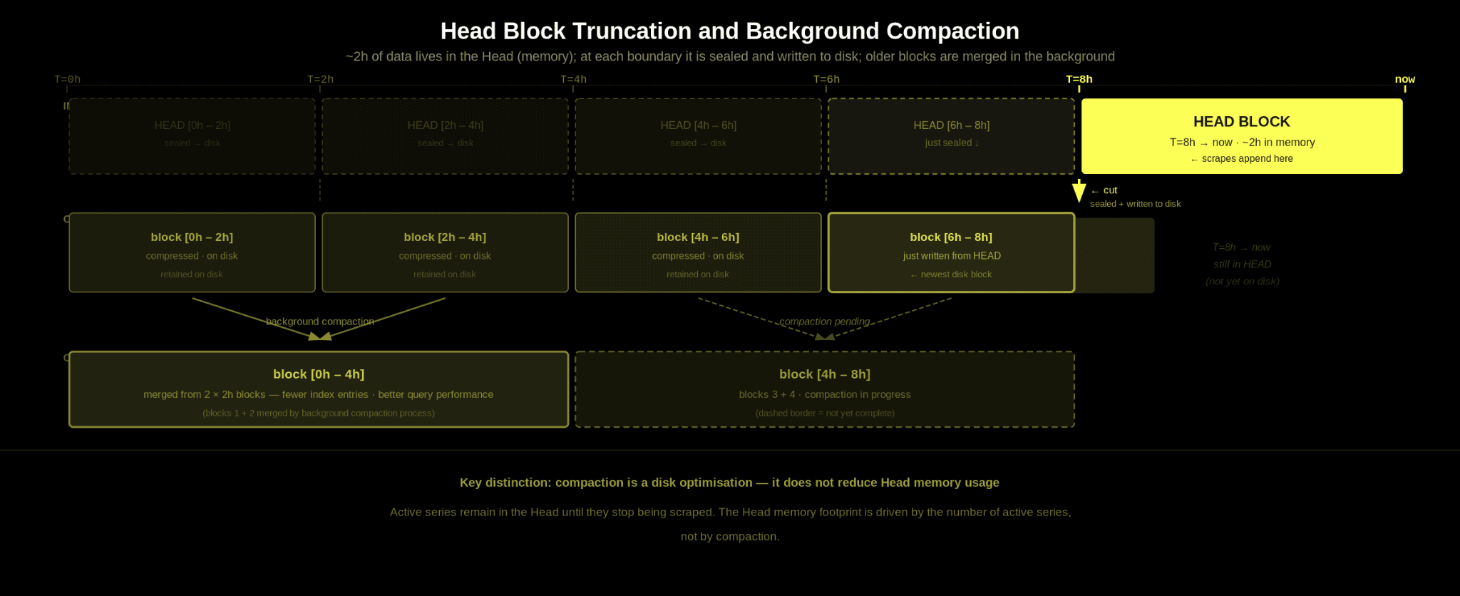
Prometheus also runs a background compaction process, similar in spirit to other LSM-style storage systems. Smaller blocks are merged into larger ones that span longer time ranges. This reduces the number of block indexes on disk and improves query efficiency by lowering per-block overhead. Compaction primarily focuses on optimizing disk layout and long-term storage efficiency. It does not directly reduce the memory overhead associated with active series in the Head.
Cleaning up memory
After chunks have been written to disk, most memSeries will still have recent chunks in memory. The Head block holds roughly 2 hours of data, and the block-cutting process is time-based and offset from the 2-hour boundary, as noted above. So series that are still receiving samples will naturally retain in-memory chunks covering the most recent window.
However, there may also be memSeries with no chunks left in memory. This can happen, for example, if a pod is restarted and the pod ID was part of the labels. In this case, the series is ephemeral; it stopped receiving data, and once its chunks were written out with a block cut, it had no in-memory samples.
After a block is cut, Prometheus performs a head truncation and cleanup pass. During this process, it looks for series that no longer have any chunks in memory and have not received recent samples, and it removes those from the in-memory index. This is effectively the point at which orphaned time series are cleaned up.
This generally ensures that short-lived series do not continue to consume memory indefinitely. That said, because block cutting and head truncation operate on a time-based cadence rather than the exact moment a series stops receiving data, a series that existed only briefly can remain in memory for a few hours before it is finally cleaned up.
Prometheus strengths
The above data model is effective when used appropriately. More specifically, when you have:
- a moderate number of long-lived series
- scraped at regular intervals, where
- values do not change dramatically between samples for a series.
In this scenario, Prometheus’s chunk compression, XOR encoding, and delta-based timestamp storage work extremely well.
Appending new values to an existing series is cheap and predictable. As long as you repeatedly scrape the same set of series and your label sets remain reasonably sized, the storage model is efficient and performs well. For these reasons, Prometheus has achieved widespread adoption and remains a successful storage engine for low-cardinality metric data.
Write-time issues with high cardinality
The weaknesses of this model appear under high cardinality and high churn.
First, there is a real overhead per series. Every time series has its own in-memory structure, including its labels, chunks, and entries in the inverted index. That overhead is manageable with a stable number of series, but it scales linearly as the number of unique series grows. More labels mean more possible combinations, and more combinations mean more series. Each one carries this overhead. It is not uncommon for the Head to consume 10s or 100s of gigabytes of RAM under cardinality explosion, leading to memory pressure or even crashes.
Labels such as container_id are particularly useful in environments like Kubernetes because they allow operators to identify issues with specific pods or container instances and preserve full-fidelity operational context. The challenge is that these labels are both high cardinality and highly ephemeral.
As workloads scale, restart, and terminate, new series are continuously created, while old ones linger in memory until cleanup. In Prometheus, this increases memory overhead and repeatedly forces the system down the more expensive series creation path rather than the cheaper append path. As a result, many teams end up stripping these dimensions, sampling them aggressively, or avoiding them entirely to prevent cardinality explosion. For example, in this post, CloudFlare detail how they use limits on new series creation to inhibit cardinality explosions
All of these factors compound, making it harder for Prometheus to perform when cardinality exceeds what the model was originally optimized for.
Aside from the technical challenges of cardinality in Prometheus, there is also a commercial impact if you’re using an observability vendor. Many vendors that use a series-based time-series data model charge based on cardinality, often per active series or per data points ingested per minute. This is because high cardinality directly increases their infrastructure costs, which they are forced to pass on to their users.
Write time compromises
Users typically respond by limiting labels, scrape frequency, or ingestion volume. Teams have to think not just about what they want to monitor, but also about how to protect Prometheus from cardinality explosion.
Aside from approaches like restricting the length of label names and the number of labels per metric, Prometheus also supports per-scrape limits. This allows you to cap the total number of samples accepted in a single scrape, with each sample potentially belonging to a different series.
While this can help prevent sudden spikes in cardinality, it does not eliminate the underlying risk. An endpoint could still emit fewer than the configured limit on each scrape while introducing new unique series over time, increasing overall cardinality and steadily consuming memory. There have been proposals to address[1][2] this with more central limits using a number of techniques.
Systems that drop data at the cardinality limit also create a release-time hazard: a new version emitting higher-cardinality metrics can knock existing series out of ingestion, breaking dashboards and alerts that were working the day before.
These measures protect Prometheus by dropping data or limiting ingestion. If a limit is reached, Prometheus simply drops samples or refuses to accept new series. Data is lost by design in order to preserve system stability.
Ultimately, the safest approach is to carefully manage cardinality from the start. Users often respond by reducing metric resolution or cardinality. This effectively means:
- Increasing the scrape interval so metrics are collected less frequently.
- Dropping certain metrics at scrape time using relabeling rules
- Reducing label dimensions to create fewer unique series.
- Limiting samples per scrape to effectively discard excess series.
You’ll find plenty of blogs and guides dedicated to managing cardinality in Prometheus. In practice, however, this creates both a cognitive and operational burden for SRE teams, who must constantly worry that a new deployment, metric, or label could suddenly introduce enough series churn to destabilize the system. More importantly, these compromises often reduce visibility into precisely the things teams most want to observe, such as individual containers, ephemeral workloads, or other high-fidelity operational dimensions.
Read time challenges
The model also has read-time tradeoffs. When Prometheus cuts blocks to disk, those blocks are memory-mapped. This is an efficient technique. The operating system only loads pages into memory when they are accessed, so idle historical data does not immediately consume heap space. For most workloads, this works well and keeps the memory footprint predictable.
If you query for a specific series, Prometheus is extremely efficient. The inverted index maps labels to series, allowing it to quickly resolve an exact label match, narrow the results to a small set of series, and read only the relevant chunks. For example, consider the following PromQL query:
rate(http_response_time_sum{
host="host-42",
application="checkout-service",
request_path="/api/payments",
status="500"
}[5m]) /
rate(http_response_time_count{
host="host-42",
application="checkout-service",
request_path="/api/payments",
status="500"
}[5m])This calculates the average response time over the last five minutes for the specific host, application, request path, and status by dividing the rate of total response time by the rate of request count.
In this case, the index lookup is precise. Very few posting lists are intersected, and only a small number of chunks are read from disk. This is a fast path. The challenge appears when queries become broader or more aggregated. Suppose you ask:
sum(rate(http_response_time_sum{
application="checkout-service",
request_path=~".+",
status=~"2..|5.."
}[5m]))
/
sum(rate(http_response_time_count{
application="checkout-service",
request_path=~".+",
status=~"2..|5.."
}[5m]))This matches all series for checkout-service, across all hosts, endpoints, and a wide range of status codes. Because the regex can expand to many possible label values, Prometheus pulls together large posting sets for endpoint and status_code, then combines them with the application constraint.
Lack of predicate pushdown
Additionally, Prometheus cannot push arbitrary value predicates down into compressed chunk storage. Once a set of series is selected, the engine must read their chunks and scan through the samples within the requested time range. You cannot say “only return values above X” and avoid reading the rest of the series. The full chunk must be decoded, even if only part of it is relevant. Targeted lookups are efficient, but broad aggregations over high-cardinality labels can load many series and decode many chunks - requiring large volumes of data to be processed.
Read time compromises
Broad queries over high-cardinality dimensions are best avoided. Queries that omit key label filters, rely heavily on regex matching, or aggregate across millions of series at once can force large postings intersections and require decoding many chunks.
In particular, wildcard-style queries across dimensions such as pod_id, container_id, or endpoint can quickly become expensive in high-churn environments. Targeted queries that narrow down label combinations perform well, but wide, high-level aggregations across large cardinality sets are where performance typically degrades.
Conclusion
High cardinality becomes challenging in Prometheus because each unique label combination creates an independent time series with its own memory, indexing, and lifecycle overhead. As dimensionality and churn increase, this impacts ingestion, querying, and operational stability, forcing users to trade off visibility, cost, and system reliability. In the next post, we’ll explore why these same workloads behave very differently in ClickHouse. In particular, we’ll look at how the wide events model, column-oriented storage, dynamic attributes, and analytical query execution fundamentally change where cardinality costs appear and why they are often far more manageable in practice.