ClickHouse Release 25.6

Another month goes by, which means it’s time for another release!

ClickHouse version 25.6 contains 25 new features 🌸 32 performance optimizations 🦋 105 bug fixes 🐝.

This release brings a single consistent snapshot across all subqueries and table references within a query, filtering by multiple projections, JSON in Parquet, and more!

A special welcome to all the new contributors in 25.6! The growth of ClickHouse's community is humbling, and we are always grateful for the contributions that have made ClickHouse so popular.

Below are the names of the new contributors:

Alexander Grueneberg, Delyan Kratunov, Denis K, Engel Danila, George Larionov, Hans Krutzer, Himanshu Pandey, Joel Höner, Kenny Sun, Krishna Mannem, Lucas Pelecq, Lucas Ricoy, Nihal Z., Nikolay Govorov, Philip Dubé, Q3Master, Roy Kim, San Tran, Sav, Shakhaev Kyamran, Tanner Bruce, abashkeev, clickhouse-gh[bot], fhw12345, haowenfeng, haoyangqian, mekpro, nihalzp, roykim98, sdairs, sinfillo

Hint: if you’re curious how we generate this list… here.

You can also view the slides from the presentation.

ClickHouse ensures that SELECT queries run on a consistent snapshot of the data. This means that for the entire duration of the query, it will see the same data, even if new rows are inserted or existing rows are updated or deleted in parallel.

At the core of this is the immutability of table data parts:

• Inserts always create new parts; existing data is never modified in place.

• Deletes and updates are eventually applied via mutations or part merges, which generate new parts with the changes applied.

Because of this immutability, SELECT queries can safely work with a consistent snapshot of the relevant data parts at the time the query starts.

The animation below illustrates this snapshot mechanism:

① When ClickHouse receives a SELECT query Q1 on table t, it identifies the relevant data parts during query planning and index analysis.

② These parts are marked as referenced by the query.

While Q1 is running, these changes can safely occur without affecting the result:

③ A part is deleted
④ A new part is inserted
⑤ A part is mutated

Thanks to the reference system, Q1 continues to read from the original snapshot and sees a fully consistent view throughout execution.

Crucially, referenced parts are not deleted until all queries using them have completed. Once Q1 finishes, its references are released and old parts can be safely cleaned up.

Before version 25.6, ClickHouse always took separate snapshots for each subquery or table reference, leading to possible inconsistencies:

① When ClickHouse receives a SELECT query with subqueries SQ1 and SQ2,

② it determines data parts for SQ1, then separately for SQ2 (④).

③ If a data part is inserted, deleted, or mutated in between,

④ the subqueries may see inconsistent versions of the data.

Since version 25.6, ClickHouse takes a single consistent snapshot across the entire query, even when it involves multiple subqueries or CTEs. This ensures correctness for even the most complex SELECTs.

This behavior is controlled by the setting enable_shared_storage_snapshot_in_query:
SET enable_shared_storage_snapshot_in_query = 1;

When enabled, all subqueries share the same snapshot for each table:

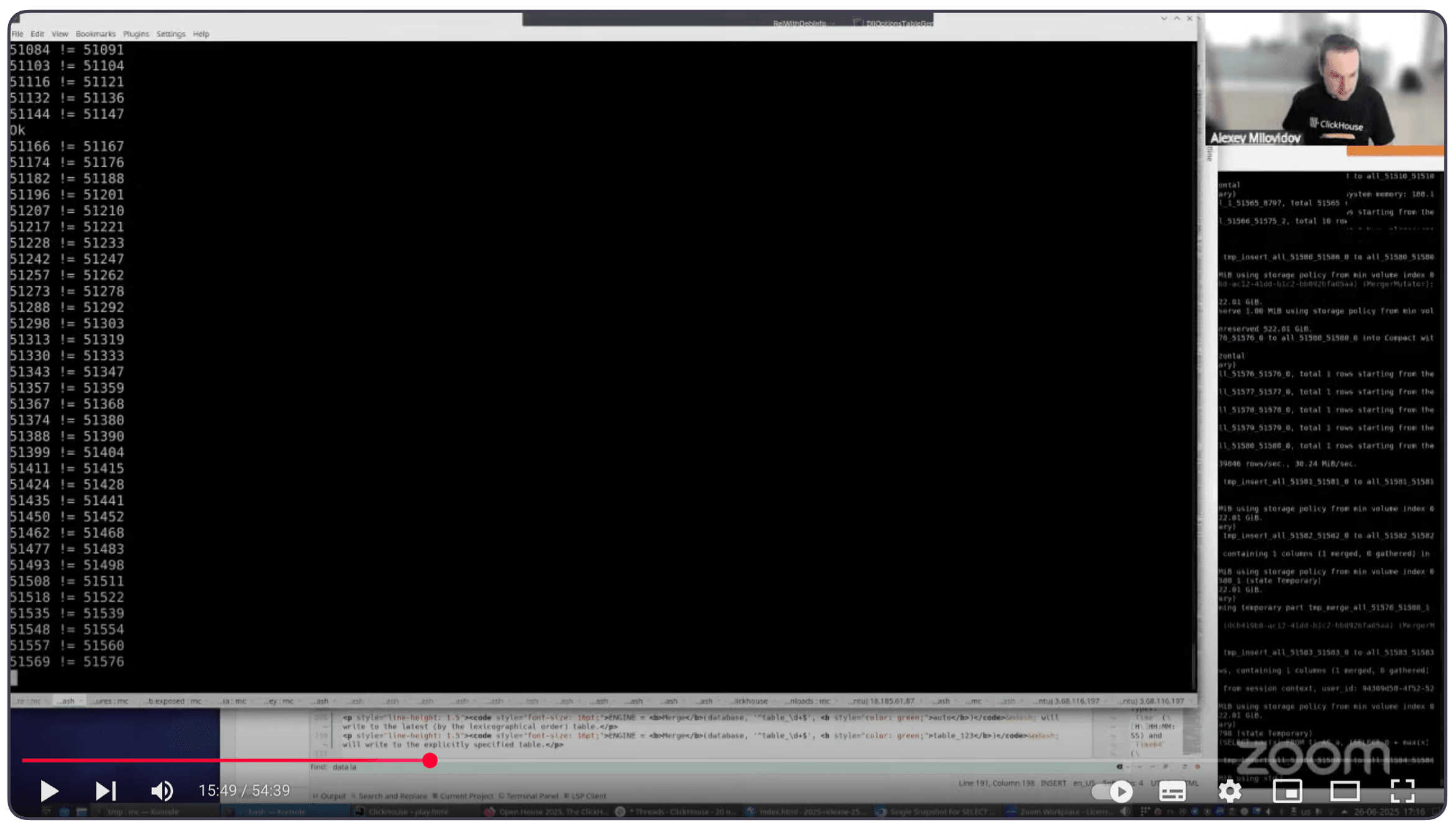
You can see the previous and this new behavior in action in the release call, where Alexey walks through a concrete example (click to open the recording at the right timecode):

ClickHouse supports several mechanisms to accelerate real-time analytics at scale. One particularly powerful feature is projections, automatically maintained, hidden tables that optimize query performance.

A projection can have a different sort order (and thus a different primary index) than the base table, and can even pre-aggregate data. When a query runs, ClickHouse automatically chooses the most efficient data path, whether from the base table or a projection, to minimize the amount of data read.

Let’s walk through a simple example with a base table and two projections:

CREATE TABLE page_views
(
    id UInt64,
    event_date Date,
    user_id UInt32,
    url String,
    region String,
    PROJECTION region_proj
    (
        SELECT * ORDER BY region
    ),
    PROJECTION user_id_proj
    (
        SELECT * ORDER BY user_id
    )
)
ENGINE = MergeTree
ORDER BY (event_date, id);

The diagram below sketches the base table and its two projections:

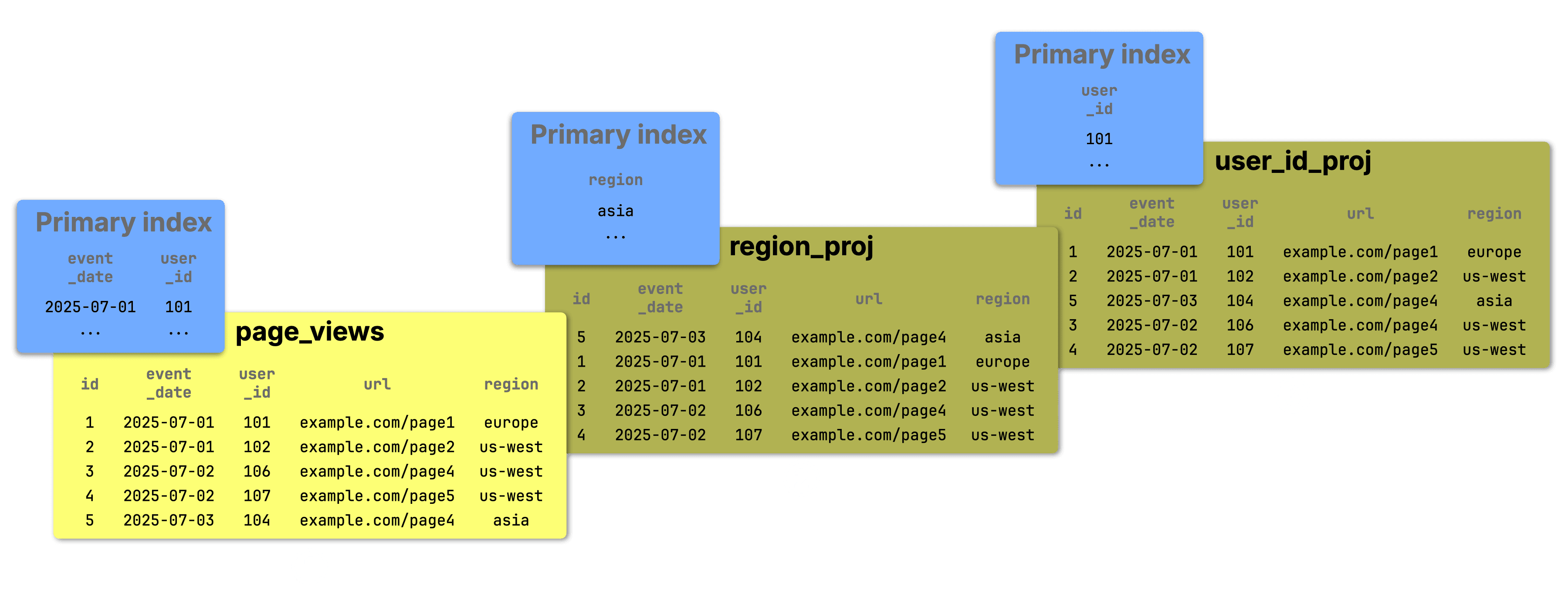
① The base table page_views tracks website visits and is sorted by (event_date, id). This defines its primary index, making queries that filter by those columns fast and efficient.

② The region_proj projection stores the same data sorted by region. Its primary index speeds up queries filtering on that column.

③ Similarly, user_id_proj stores the data sorted by user_id, optimizing for queries on that field.

Previously, projections had two main limitations:

1. Each projection duplicated the full base table data, leading to storage overhead.

2. Only one projection could be used per query, limiting optimization when multiple filters were involved.

Since version 25.5, ClickHouse supports the virtual column _part_offset in projections. This unlocks a more space-efficient way to store projections.

There are now two ways to define a projection:

1. Store full columns (the original behavior): The projection contains full data and can be read directly, offering faster performance when filters match the projection’s sort order.

2. Store only the sorting key + _part_offset: The projection works like an index. ClickHouse uses the projection’s primary index to locate matching rows, but reads the actual data from the base table. This reduces storage overhead at the cost of slightly more I/O at query time.

You can also mix these approaches, storing some columns in the projection and others indirectly via _part_offset.

The diagram below illustrates the second (index-like) approach:

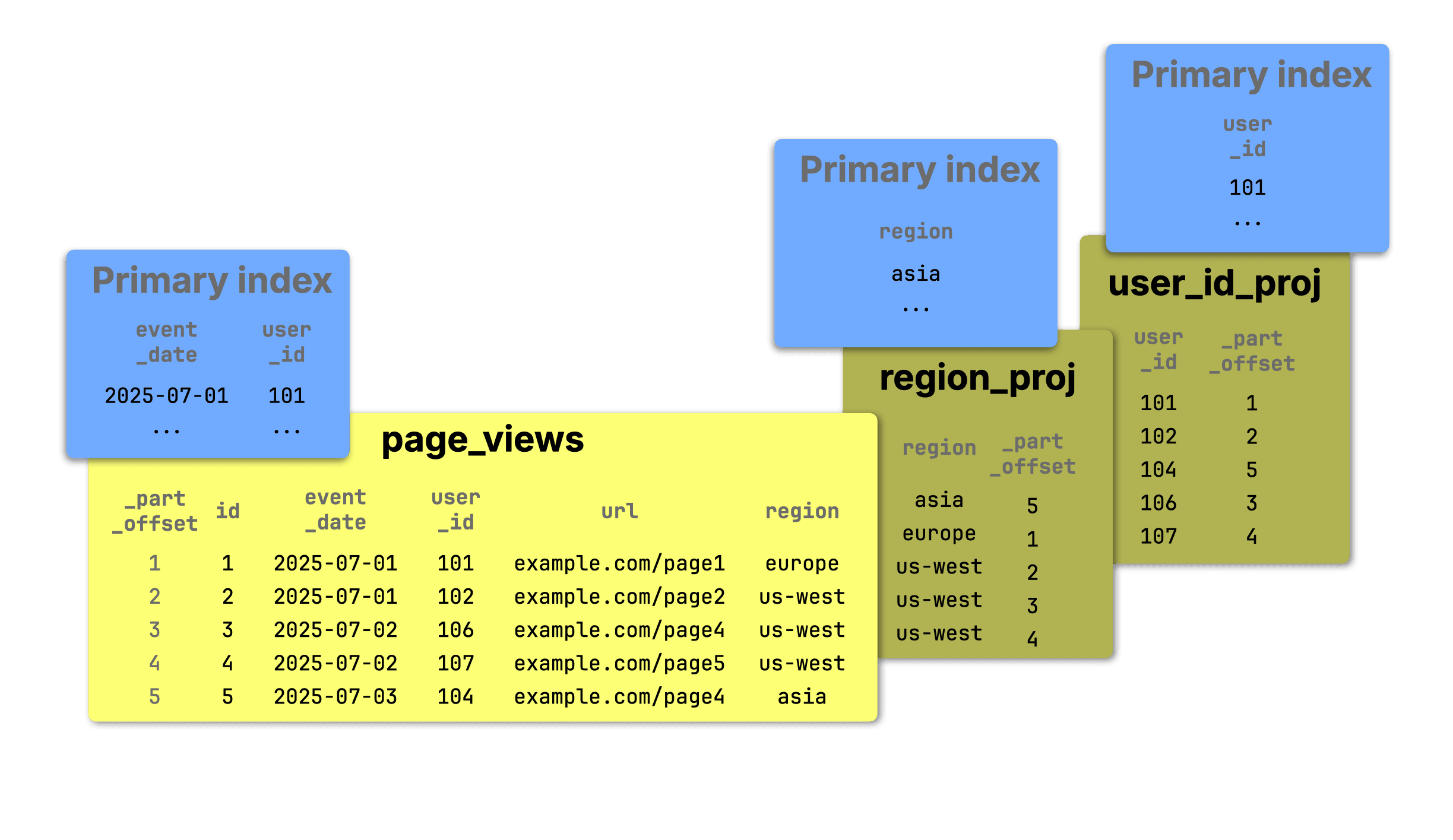
① The base table now shows the virtual _part_offset column.

② The region_proj and ③ user_id_proj projections store only their sorting key and _part_offset, referencing rows in the base table and significantly reducing data duplication.

Starting in version 25.6, building on the _part_offset support introduced in the previous version, ClickHouse can now use multiple projections to accelerate a single query with multiple filters.

Importantly, ClickHouse still reads data from only one projection (or the base table), but can use other projections' primary indexes to prune unnecessary parts before reading.

This is especially useful for queries that filter on multiple columns, each potentially matching a different projection.

Currently, this mechanism only prunes entire parts. Granule-level pruning is not yet supported.

To demonstrate this, we define the table (with projections using _part_offset columns) and insert five example rows matching the diagrams above.

CREATE TABLE page_views
(
    id UInt64,
    event_date Date,
    user_id UInt32,
    url String,
    region String,
    PROJECTION region_proj
    (
        SELECT _part_offset ORDER BY region
    ),
    PROJECTION user_id_proj
    (
        SELECT _part_offset ORDER BY user_id
    )
)
ENGINE = MergeTree
ORDER BY (event_date, id);
SETTINGS
    index_granularity = 1, -- one row per granule
    max_bytes_to_merge_at_max_space_in_pool = 1; -- disable merge

INSERT INTO page_views VALUES (
1, '2025-07-01', 101, 'https://example.com/page1', 'europe');
INSERT INTO page_views VALUES (
2, '2025-07-01', 102, 'https://example.com/page2', 'us_west');
INSERT INTO page_views VALUES (
3, '2025-07-02', 106, 'https://example.com/page3', 'us_west');
INSERT INTO page_views VALUES (
4, '2025-07-02', 107, 'https://example.com/page4', 'us_west');
INSERT INTO page_views VALUES (
5, '2025-07-03', 104, 'https://example.com/page5', 'asia');

Note: The table uses custom settings for illustration, such as one-row granules and disabled part merges, which are not recommended for production use.

This setup produces:

• 5 separate parts (one per inserted row)

• One primary index entry per row (in the base table and each projection)

• Each part contains exactly one row

With this setup, we run a query filtering on both region and user_id (shown below). Since the base table’s primary index based on the compound sorting key (event_date, id) is unhelpful here, ClickHouse uses:

• region_proj to prune parts by region

• user_id_proj to further prune by user_id

This behavior is visible via EXPLAIN projections = 1, which shows how ClickHouse selects and applies projections.

EXPLAIN projections=1
SELECT * FROM page_views WHERE region = 'us_west' AND user_id = 107;

Expression ((Project names + Projection))
  Expression
①  ReadFromMergeTree (default.page_views)
    Projections:
②     Name: region_proj
        Description: Projection has been analyzed and is used for part-level filtering
        Condition: (region in ['us_west', 'us_west'])
        Search Algorithm: binary search
        Parts: 3
        Marks: 3
        Ranges: 3
        Rows: 3
        Filtered Parts: 2
③     Name: user_id_proj
        Description: Projection has been analyzed and is used for part-level filtering
        Condition: (user_id in [107, 107])
        Search Algorithm: binary search
        Parts: 1
        Marks: 1
        Ranges: 1
        Rows: 1
        Filtered Parts: 2

The EXPLAIN output (shown above) reveals the logical query plan, top to bottom:

• ① Plans to read from the page_views base table

• ② Uses region_proj to identify 3 parts where region = 'us_west', pruning 2 of the 5 parts

• ③ Uses user_id_proj to identify 1 part where user_id = 107, further pruning 2 of the 3 remaining parts

In the end, just 1 out of 5 parts is read from the base table.

By combining the index analysis of multiple projections, ClickHouse significantly reduces the amount of data scanned, improving performance while keeping storage overhead low.

Parquet doesn’t fully support the JSON datatype. Instead, it has a logical JSON type that physically stores the data as a string with an annotation. Or as described in the docs:

It must annotate a BYTE_ARRAY primitive type. The BYTE_ARRAY data is interpreted as a UTF-8 encoded character string of valid JSON as defined by the JSON specification

Let’s have a look at how this works by writing the ClickHouse JSON type to a Parquet file:

1SELECT '{"database": "ClickHouse", "is_it_good": true}'::JSON AS data
2INTO OUTFILE 'test.parquet';

We can use the ParquetMetadata input format when parsing the file:

1SELECT *
2FROM file('test.parquet', ParquetMetadata)
3FORMAT PrettyJSONEachRow;

{
    "num_columns": "1",
    "num_rows": "1",
    "num_row_groups": "1",
    "format_version": "2",
    "metadata_size": "232",
    "total_uncompressed_size": "174",
    "total_compressed_size": "206",
    "columns": [
        {
            "name": "data",
            "path": "data",
            "max_definition_level": "0",
            "max_repetition_level": "0",
            "physical_type": "BYTE_ARRAY",
            "logical_type": "JSON",
            "compression": "ZSTD",
            "total_uncompressed_size": "174",
            "total_compressed_size": "206",
            "space_saved": "-18.39%",
            "encodings": [
                "PLAIN",
                "RLE_DICTIONARY"
            ]
        }
    ],
    "row_groups": [
        {
            "file_offset": "4",
            "num_columns": "1",
            "num_rows": "1",
            "total_uncompressed_size": "174",
            "total_compressed_size": "206",
            "columns": [
                {
                    "name": "data",
                    "path": "data",
                    "total_compressed_size": "206",
                    "total_uncompressed_size": "174",
                    "have_statistics": true,
                    "statistics": {
                        "num_values": "1",
                        "null_count": null,
                        "distinct_count": null,
                        "min": "{\"database\":\"ClickHouse\",\"is_it_good\":true}",
                        "max": "{\"database\":\"ClickHouse\",\"is_it_good\":true}"
                    },
                    "bloom_filter_bytes": "47"
                }
            ]
        }
    ]
}

Under columns, we can see a logical_type of JSON and a physical_type of BYTE_ARRAY, as expected.

In ClickHouse 25.5 and earlier, we would read the logical JSON type back as a String:

1select *, * APPLY(toTypeName) 
2FROM file('test.parquet');

┌─data────────────────────────────────────────┬─toTypeName(data)─┐
│ {"database":"ClickHouse","is_it_good":true} │ Nullable(String) │
└─────────────────────────────────────────────┴──────────────────┘

That’s no longer the case in ClickHouse 25.6, where the data will now be read back into the JSON data type:

┌─data────────────────────────────────────────┬─toTypeName(data)─┐
│ {"database":"ClickHouse","is_it_good":true} │ JSON             │
└─────────────────────────────────────────────┴──────────────────┘

For better compatibility with other SQL DBMS, ClickHouse now has Time and Time64 data types, which allow you to store time values.

Time stores times down to the second (with a range of [-999:59, 999:59]), taking up 32 bits per value, and Time64 stores time down to the sub-second (with a range of [-999:59.999999999, 999:59.99999999]), taking up 64 bits per value.

This is an experimental feature at the moment, so you need to set the enable_time_time64_type property to use it:

1SET enable_time_time64_type=1;

We can then cast the output of now() to Time to extract the current time:

1SELECT now()::Time;

┌─CAST(now(), 'Time')─┐
│            13:38:25 │
└─────────────────────┘

Or maybe we want to store our running metrics:

CREATE TABLE runningTimes(
  time Time64(3)
)
ORDER BY time;

INSERT INTO runningTimes VALUES ('00:07:45.143') ('00:08:02.001') ('00:07:42.001');

If we want to find the average time, we can’t currently do this directly on the Time data type (but it is in progress). However, we can convert the times to UInt32 and compute the aggregation before casting back:

1select avg(toUInt32(time))::Time AS avg 
2FROM runningTimes;

┌──────avg─┐
│ 00:07:49 │
└──────────┘

We have two new system tables:

• system.codecs, which provides documentation for ClickHouse’s compression and encryption codecs
• iceberg_history, which contains information about all available snapshots of Apache Iceberg tables.

First, let’s look at the system.codecs table:

1DESCRIBE system.codecs;

┌─name───────────────────┬─type───┐
│ name                   │ String │
│ method_byte            │ UInt8  │
│ is_compression         │ UInt8  │
│ is_generic_compression │ UInt8  │
│ is_encryption          │ UInt8  │
│ is_timeseries_codec    │ UInt8  │
│ is_experimental        │ UInt8  │
│ description            │ String │
└────────────────────────┴────────┘

We can then write the following query to return the name and description of some of the codecs:

1SELECT name, description 
2FROM system.codecs
3LIMIT 3
4FORMAT Vertical;

Row 1:
──────
name:        GCD
description: Preprocessor. Greatest common divisor compression; divides values by a common divisor; effective for divisible integer sequences.

Row 2:
──────
name:        AES_128_GCM_SIV
description: Encrypts and decrypts blocks with AES-128 in GCM-SIV mode (RFC-8452).

Row 3:
──────
name:        FPC
description: High Throughput Compression of Double-Precision Floating-Point Data

Next, for Iceberg users, the system.iceberg_history table has the following structure:

1DESCRIBE TABLE system.iceberg_history

┌─name────────────────┬─type────────────────────┐
│ database_name       │ String                  │
│ table_name          │ String                  │
│ made_current_at     │ Nullable(DateTime64(6)) │
│ snapshot_id         │ UInt64                  │
│ parent_id           │ UInt64                  │
│ is_current_ancestor │ UInt8                   │
└─────────────────────┴─────────────────────────┘

We can then time travel by writing queries that use made_current_at or snapshot_id

This one-line fix might have saved OpenAI’s cluster, and a few engineers’ heart rates.

During the launch of GPT-4o’s image generation, when the internet was busy turning everything from pets to profile pics into Studio Ghibli characters, OpenAI’s observability system was hit with a massive traffic surge. Log volume spiked by 50% overnight. CPU usage shot through the roof.

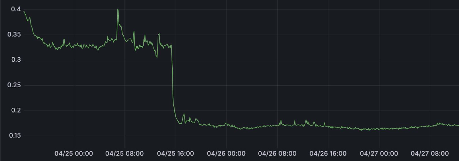
The culprit for the CPU usage? An expensive division operation buried deep inside ClickHouse’s Bloom filter index code, executed every time an element was inserted. OpenAI engineer Delyan Kratunov spotted it and replaced the division with a fast multiplication and bit shift.

The result? A 40% drop in CPU usage with a near one-line change. Crisis averted. Cluster saved. And now, thanks to Delyan, the whole community gets the benefit in 25.6.

You can read the full story in OpenAI’s user story about why they chose ClickHouse for observability at mind-bending scale.

Thanks again to Delyan and the OpenAI team for upstreaming the fix! 🌸

Last but not least, every ClickHouse installation now comes bundled with a powerful new command-line tool for monitoring and diagnostics: chdig.

You can launch it like any other ClickHouse tool: clickhouse-chdig, clickhouse chdig, or simply chdig.

It’s a top-like TUI interface designed specifically for ClickHouse, offering deep insights into how your queries and servers behave in real time.

Here are just a few things it can do:

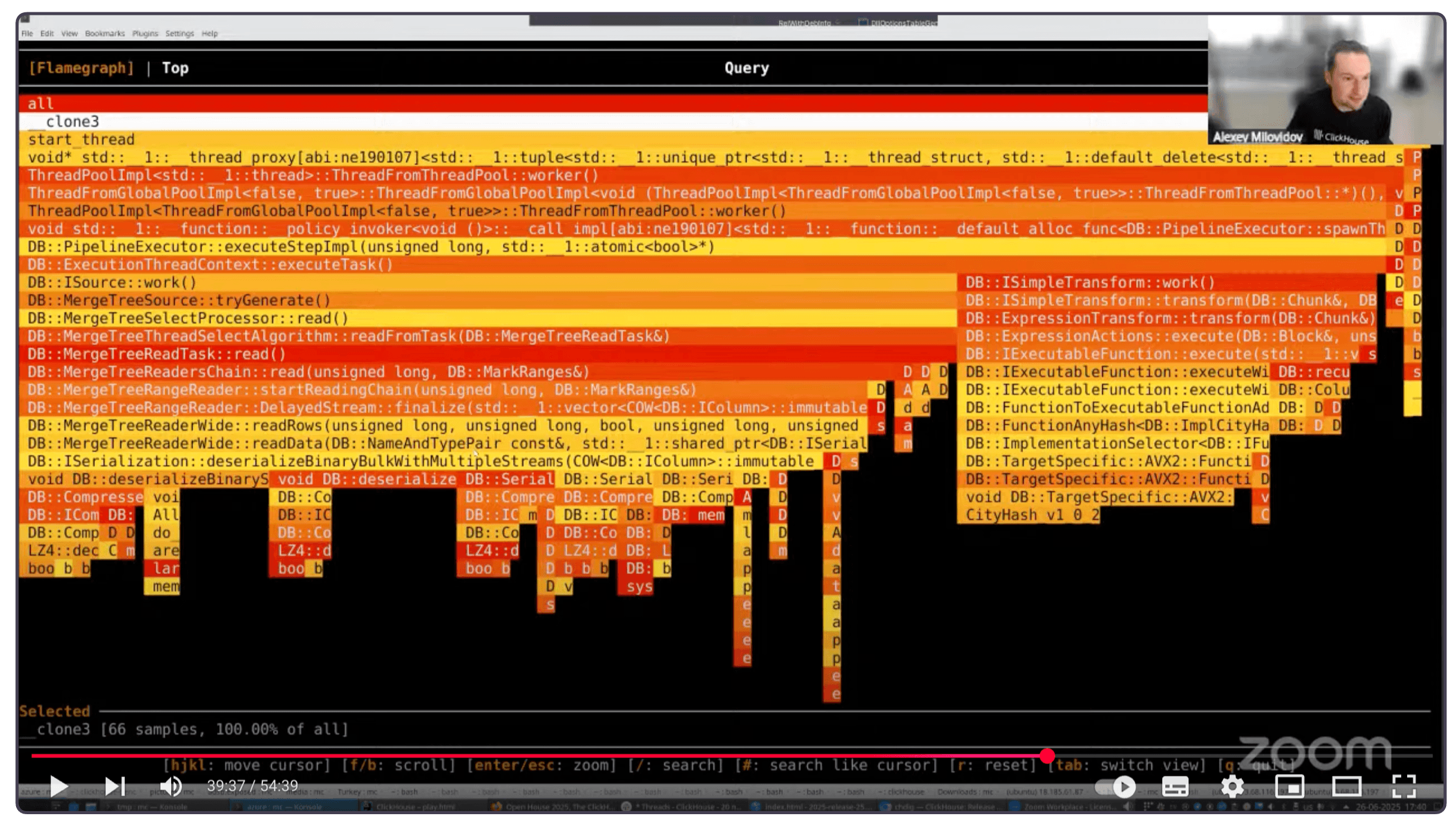
• Flamegraphs, everywhere
  View CPU, memory, and real-time flamegraphs to understand query performance bottlenecks and internal behavior, with interactive speedscope support built in.

• Understand query internals at a glance
  Jump into views for query processors, pipelines, logs, system tables, query plans, and even kill misbehaving queries with one key.

• Cluster-aware & history-enabled
  Monitor an entire cluster at once, or step back in time using historical logs from rotated system.log tables.

To get a sense of how it works, here’s Alexey demoing it at the release call (click to open the recording at the right timecode):