Introduction
Here at ClickHouse, we consider Observability to be just another real-time analytics problem. As a high-performance real-time analytics database, ClickHouse is used for many use cases, including real-time analytics for time series data. Its diversity of use cases has helped drive a huge range of analytical functions, which assist in querying most data types. These query features and high compression rates have increasingly led users to utilize ClickHouse to store Observability data. This data takes three common forms: logs, metrics, and traces. In this blog, the second in an Observability series, we explore how trace data can be collected, stored, and queried in ClickHouse.
We have focused this post on using OpenTelemetry to collect trace data for storage in ClickHouse. When combined with Grafana, and recent developments in the ClickHouse plugin, traces are easily visualized and can be combined with logs and metrics to obtain a deep understanding of your system behavior and performance when detecting and diagnosing issues.
We have attempted to ensure that any examples can be reproduced, and while this post focuses on data collection and visualization basics, we have included some tips on schema optimization. For example purposes, we have forked the official OpenTelemetry Demo, adding support for ClickHouse and including an OOTB Grafana dashboard for visualizing traces.
What are Traces?
Telemetry is data emitted from a system about its behavior. This data can take the form of logs, metrics, and traces. A trace records the paths taken by requests (made by an application or end-user) as they propagate through multi-service architectures such as microservice and serverless applications. A single trace consists of multiple spans, each a unit of work or operation. The span provides details of an operation, principally the time it took, in addition to other metadata and related log messages. These spans are hierarchy related as a tree, with the first span relating the root and covering the entire trace from start to finish. Beneath this root and each subsequent span, child operations are captured. As we navigate the tree, we can see the child operations and steps that make up the above level. This gives us ever-increasing context as to the work performed by the original request. This is visualized below:

These traces, when combined with metrics and logs, can be critical in obtaining insights into the behavior of a system for the detection and resolution of issues.
What is OpenTelemetry?
The OpenTelemetry project is a vendor-neutral open-source framework consisting of SDKs, APIs, and components that allow the ingesting, transforming, and sending of Observability data to a backend. More specifically, this consists of several main components:
- A set of specifications and conventions of how metrics, logs, and traces should be collected and stored. This includes recommendations for language-specific agents and a full specification for the OpenTelemetry Line Protocol (OTLP) based on protobuf. This allows data to be transmitted between services by providing a full description of the client-server interface and the message format.
- Language-specific libraries and SDKs for instrumenting, generating, collecting, and exporting observability data. This is particularly relevant to the collection of trace data.
- An OTEL Collector written in Golang provides a vendor-agnostic implementation of receiving, processing and exporting Observability data. The OTEL Collector provides a centralized processing gateway by supporting several input formats, such as Prometheus and OTLP, and a wide range of export targets, including ClickHouse.
In summary, OpenTelemetry standardizes the collection of logs, metrics, and traces. Importantly, it is not responsible for storing this data in an Observability backend - this is where ClickHouse comes in!
Why ClickHouse?
Trace data is typically represented as a single table, with each span a row, and thus can be considered just another real-time analytics problem. As well as providing high compression for this data type, ClickHouse provides a rich SQL interface with additional analytical functions that trivialize querying traces. When combined with Grafana, users have a highly cost-efficient way of storing and visualizing traces. While other stores may offer similar compression levels, ClickHouse is unique in combining this low latency querying as the world's fastest analytical database. In fact, these characteristics led to ClickHouse becoming a preferred backend for many commercial observability solutions like: Signoz.io, Highlight.io, qryn, BetterStack, or homegrown large-scale observability platforms like Uber, Cloudflare, or Gitlab.
Instrumentation Libraries
Instrumentation libraries are provided for the most popular languages. These provide both automatic instrumentation of code, where an application/services framework is exploited to capture the most common metric and trace data, and manual instrumentation techniques. While automatic instrumentation is typically sufficient, the latter allows users to instrument-specific parts of their code, potentially in more detail - capturing application-specific metrics and trace information.
For the purposes of this blog, we are only interested in the capture of trace information. The OpenTelemetry demo application consists of a microservices architecture with many dependent services, each in a different language, to provide a reference for implementors. The simple example below shows the instrumentation of a Python Flask API to collect trace data:
# These are the necessary import declarations
from opentelemetry import trace
from random import randint
from flask import Flask, request
# Acquire a tracer
tracer = trace.get_tracer(__name__)
app = Flask(__name__)
@app.route("/rolldice")
def roll_dice():
return str(do_roll())
def do_roll():
# This creates a new span that's the child of the current one
with tracer.start_as_current_span("do_roll") as rollspan:
res = randint(1, 6)
rollspan.set_attribute("roll.value", res)
return resA detailed guide on each library is well beyond the scope of this blog, and we encourage users to read the relevant documentation for their language.
OTEL Collector
The OTEL collector accepts data from Observability sources, such as trace data from an instrumentation library, processes this data, and exports it to the target backend. The OTEL Collector can also provide a centralized processing gateway by supporting several input formats, such as Prometheus and OTLP, and a wide range of export targets, including ClickHouse.
The Collector uses the concept of pipelines. These can be of type logs, metrics, or traces and consist of a receiver, processor, and exporter.

The receiver in this architecture acts as the input for OTEL data. This can be either via a pull or push model. While this can occur over a number of protocols, trace data from instrumentation libraries will be pushed via OTLP using either gRPC or HTTP. Processors subsequently run on this data providing filtering, batching, and enrichment capabilities. Finally, an exporter sends the data to a backend destination via either push or pull. In our case, we will push the data to ClickHouse.
Note that while more commonly used as a gateway/aggregator, handling tasks such as batching and retries, the collector can also be deployed as an agent itself - this is useful for log collection, as described in our previous post. OTLP represents the OpenTelemetry data standard for communication between gateway and agent instances, which can occur over gRPC or HTTP. For the purposes of trace collection, the collector is simply deployed as a gateway, however, as shown below:

Note that more advanced architectures are possible for higher load environments. We recommend this excellent video discussing possible options.
ClickHouse Support
ClickHouse is supported in the OTEL exporter through a community contribution, with support for logs, traces, and metrics. Communication with ClickHouse occurs over the optimized native format and protocol via the official Go client. Before using the OpenTelemetry Collector, users should consider the following points:
-
The ClickHouse data model and schema that the agent uses are hard coded. As of the time of writing, there is no ability to change the types or codecs used. Mitigate this by creating the table before deploying the connector, thus enforcing your schema.
-
The exporter is not distributed with the core OTEL distribution but rather as an extension through the
contribimage. Practically this means using the correct Docker image in any HELM chart. For leaner deployments, users can build a custom collector image with only the required components. -
As of version 0.74, users should pre-create the database in ClickHouse before deployment if not set to the value of
default(as used in the demo fork).CREATE DATABASE otel -
The exporter is in alpha, and users should adhere to the advice provided by OpenTelemetry.
Example Application

OpenTelemetry provides a demo application giving a practical example of the implementation of OpenTelemetry. This is a distributed micro-services architecture that powers a web store selling telescopes. This e-commerce use-case is useful in creating an opportunity for a wide range of simple, understandable services, e.g., recommendations, payments, and currency conversion. The storefront is subjected to a load generator, which causes each instrumented service to generate logs, traces, and metrics. As well as providing a realistic example for practitioners to learn how to instrument in their preferred language, this demo also allows vendors to show off their OpenTelemetry integration with their Observability backend. In this spirit, we have forked this application and made the necessary changes to store trace data in ClickHouse.
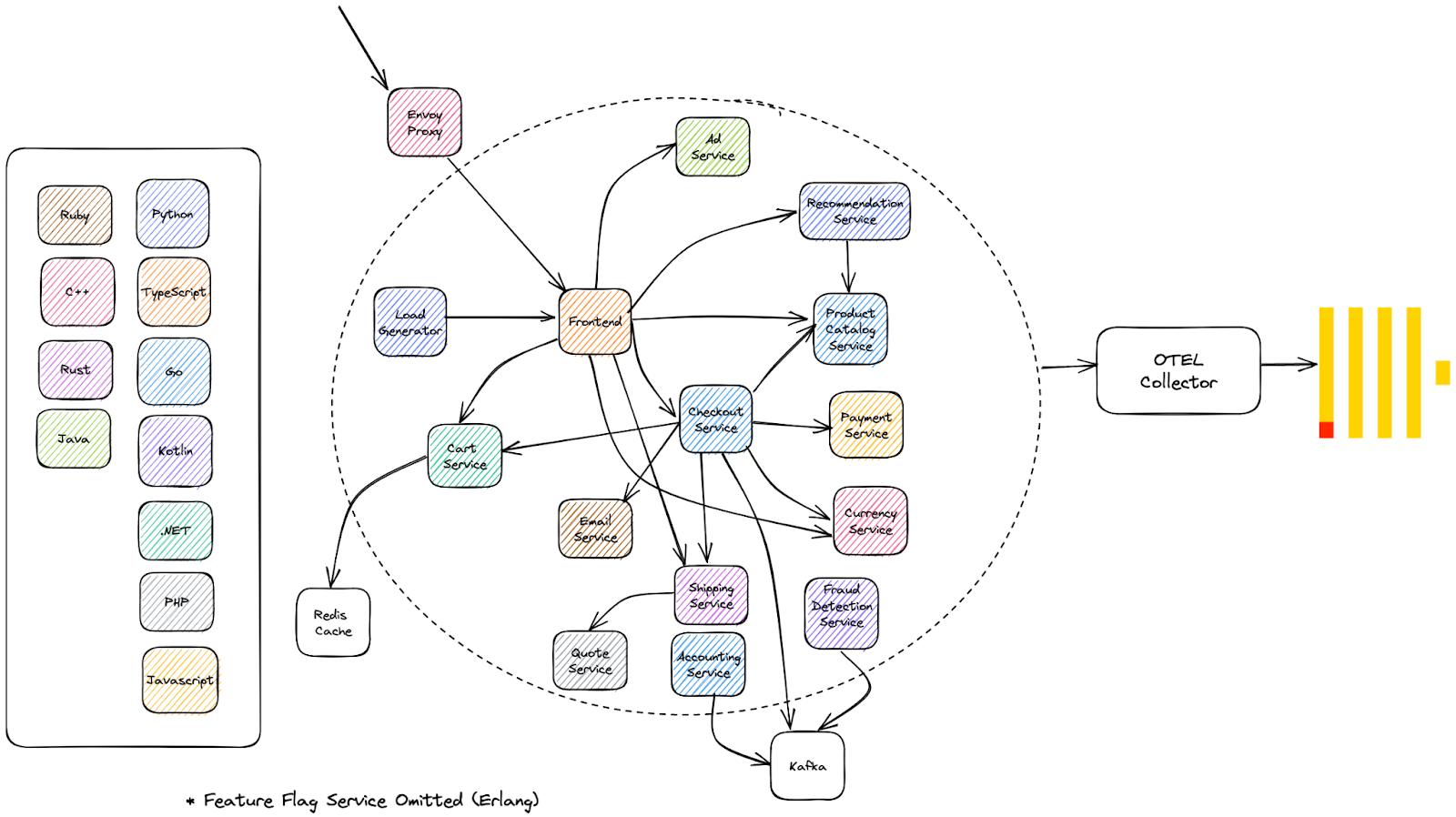
Note the breadth of languages used in the above architecture and the number of components handling operations such as payments and recommendations. Users are recommended to check the code for the service in their preferred language. Due to the presence of a collector as a gateway, no changes have been made to any instrumentation code. This architectural separation is one of the clear benefits of OpenTelemetry - backends can be changed with just a change of the target exporter in the collector.
Deploying Locally
The demo uses a Docker container for each service. The demo can be deployed using docker compose and the steps outlined in the official documentation, substituting the ClickHouse fork for the original repository.
git clone https://github.com/ClickHouse/opentelemetry-demo.git
cd opentelemetry-demo/
docker compose up --no-buildWe have modified the docker-compose file to include a ClickHouse instance in which data will be stored, available to the other services as clickhouse.
Deploying with Kubernetes
The demo can easily be deployed in Kubernetes using the official instructions. We recommend copying the values file and modifying the collector configuration. A sample values file, which sends all spans to a ClickHouse Cloud instance, can be found here. This can be downloaded and deployed with a modified helm command, i.e.,
helm install -f values.yaml my-otel-demo open-telemetry/opentelemetry-demoIntegrating ClickHouse
In this post, we focus on exporting traces only. While logs and metrics can also be stored in ClickHouse, we use the default configuration for simplicity. Logs are not enabled by default, and metrics are sent to Prometheus.
To send trace data to ClickHouse, we must add a custom OTEL Collector configuration via the file otel-config-extras.yaml. This will be merged with the main configuration, overriding any existing declarations. The additional configuration is shown below:
exporters:
clickhouse:
endpoint: tcp://clickhouse:9000?dial_timeout=10s&compress=lz4
database: default
ttl_days: 3
traces_table_name: otel_traces
timeout: 5s
retry_on_failure:
enabled: true
initial_interval: 5s
max_interval: 30s
max_elapsed_time: 300s
processors:
batch:
timeout: 5s
send_batch_size: 100000
service:
pipelines:
traces:
receivers: [otlp]
processors: [spanmetrics, batch]
exporters: [logging, clickhouse]The main changes here are configuring ClickHouse as an exporter. A few key settings here:
- The endpoint setting specifies the ClickHouse host and port. Note communication occurs over TCP (port 9000). For secure connections, this should be 9440 with a
secure=trueparameter, e.g.,'clickhouse://<username>:<password>@<host>:9440?secure=true'. Alternatively, use thedsnparameter. Note we connect to hostclickhousehere. This is the clickhouse container, added to the local deployment docker image. Feel free to modify this path, e.g., to point to a ClickHouse Cloud cluster. ttl_days- This controls data retention in ClickHouse via the TTL feature. See the section "Schema" below.
Our traces pipeline utilizes the OTLP receiver to receive trace data from the instrumentation libraries. This pipeline then passes this data to two processors:
- A batch processor is responsible for ensuring INSERTs occur at most every 5s or when the batch size reaches 100k. This ensures inserts are batched efficiently.
- A spanmetrics processor. This aggregates request, error, and metrics from trace data, forwarding it to the metrics pipeline. We will utilize this in a later post on metrics.
Schema
Once deployed, we can confirm trace data is being sent to ClickHouse using a simple SELECT on the table otel_traces. This represents the main data to which all spans are sent. Note we access the container using the clickhouse-client (it should be exposed on the host on the default 9000 port).
SELECT *
FROM otel_traces
LIMIT 1
FORMAT Vertical
Row 1:
──────
Timestamp: 2023-03-20 18:04:35.081853291
TraceId: 06cabdd45e7c3c0172a8f8540e462045
SpanId: b65ebde75f6ae56f
ParentSpanId: 20cc5cb86c7d4485
TraceState:
SpanName: oteldemo.AdService/GetAds
SpanKind: SPAN_KIND_SERVER
ServiceName: adservice
ResourceAttributes: {'telemetry.auto.version':'1.23.0','os.description':'Linux 5.10.104-linuxkit','process.runtime.description':'Eclipse Adoptium OpenJDK 64-Bit Server VM 17.0.6+10','service.name':'adservice','service.namespace':'opentelemetry-demo','telemetry.sdk.version':'1.23.1','process.runtime.version':'17.0.6+10','telemetry.sdk.name':'opentelemetry','host.arch':'aarch64','host.name':'c97f4b793890','process.executable.path':'/opt/java/openjdk/bin/java','process.pid':'1','process.runtime.name':'OpenJDK Runtime Environment','container.id':'c97f4b7938901101550efbda3c250414cee6ba9bfb4769dc7fe156cb2311735e','os.type':'linux','process.command_line':'/opt/java/openjdk/bin/java -javaagent:/usr/src/app/opentelemetry-javaagent.jar','telemetry.sdk.language':'java'}
SpanAttributes: {'thread.name':'grpc-default-executor-1','app.ads.contextKeys':'[]','net.host.name':'adservice','app.ads.ad_request_type':'NOT_TARGETED','rpc.method':'GetAds','net.host.port':'9555','net.sock.peer.port':'37796','rpc.service':'oteldemo.AdService','net.transport':'ip_tcp','app.ads.contextKeys.count':'0','app.ads.count':'2','app.ads.ad_response_type':'RANDOM','net.sock.peer.addr':'172.20.0.23','rpc.system':'grpc','rpc.grpc.status_code':'0','thread.id':'23'}
Duration: 218767042
StatusCode: STATUS_CODE_UNSET
StatusMessage:
Events.Timestamp: ['2023-03-20 18:04:35.145394083','2023-03-20 18:04:35.300551833']
Events.Name: ['message','message']
Events.Attributes: [{'message.id':'1','message.type':'RECEIVED'},{'message.id':'2','message.type':'SENT'}]
Links.TraceId: []
Links.SpanId: []
Links.TraceState: []
Links.Attributes: []Each row represents a span, some of which are also root spans. There are some key fields, which with a basic understanding, will allow us to construct useful queries. A full description of trace metadata is available here:
- TraceId - The Trace Id represents the trace that the Span is a part of.
- SpanId - A Span's unique Id
- ParentSpanId - The span id of the Span’s parent span. This allows a trace call history to be constructed. This will be empty for root spans.
- SpanName - the name of the operation
- SpanKind - When a span is created, its Kind is either a Client, Server, Internal, Producer, or Consumer. This Kind hints to the tracing backend as to how the trace should be assembled. It effectively describes the relationship of the Span to its children and parents.
- ServiceName - the name of the service, e.g., Adservice, from which the Span originates.
- ResourceAttributes - key-value pairs that contain metadata that you can use to annotate a Span to carry information about the operation it is tracking. This might, for example, contain Kubernetes information, e.g., pod name or values concerning the host. Note our schema forces keys and values to be both String with a Map type.
- SpanAttributes - additional span level attributes, e.g.,
thread.id. - Duration - duration of the Span in nanoseconds.
- StatusCode - Either UNSET, OK, or ERROR. The latter will be set when there is a known error in the application code, such as an exception.
- Events* - While possibly inappropriate for dashboard overviews, these can interest the application developer. This can be thought of as a structured annotation on a Span, typically used to denote a meaningful, singular point during the Span’s duration, e.g., when a page becomes interactive. The
Events.Timestamp,Events.Name, andEvents.Attributescan be used to reconstruct the full event - note this relies on array positions. - Links* - These imply a casual relationship to another span. For example, these might be asynchronous operations executed as a result of this specific operation. A processing job that is queued due to a request operation might be an appropriate span link. Here the developer might link the last Span from the first trace to the first Span in the second trace to causally associate them. In the ClickHouse schema, we again rely on Array types and associating the positions of the columns
Links.TraceId,Links.SpanId, andLinks.Attributes.
Note that the collector is opinionated on the schema, including enforcing specific codecs. While these represent sensible choices for the general case, they prevent users from tuning the configuration to their needs via collector configuration. Users wishing to modify the codecs or the ORDER BY key, e.g., fit user-specific access patterns, should pre-create the table in advance.
CREATE TABLE otel_traces
(
`Timestamp` DateTime64(9) CODEC(Delta(8), ZSTD(1)),
`TraceId` String CODEC(ZSTD(1)),
`SpanId` String CODEC(ZSTD(1)),
`ParentSpanId` String CODEC(ZSTD(1)),
`TraceState` String CODEC(ZSTD(1)),
`SpanName` LowCardinality(String) CODEC(ZSTD(1)),
`SpanKind` LowCardinality(String) CODEC(ZSTD(1)),
`ServiceName` LowCardinality(String) CODEC(ZSTD(1)),
`ResourceAttributes` Map(LowCardinality(String), String) CODEC(ZSTD(1)),
`SpanAttributes` Map(LowCardinality(String), String) CODEC(ZSTD(1)),
`Duration` Int64 CODEC(ZSTD(1)),
`StatusCode` LowCardinality(String) CODEC(ZSTD(1)),
`StatusMessage` String CODEC(ZSTD(1)),
`Events.Timestamp` Array(DateTime64(9)) CODEC(ZSTD(1)),
`Events.Name` Array(LowCardinality(String)) CODEC(ZSTD(1)),
`Events.Attributes` Array(Map(LowCardinality(String), String)) CODEC(ZSTD(1)),
`Links.TraceId` Array(String) CODEC(ZSTD(1)),
`Links.SpanId` Array(String) CODEC(ZSTD(1)),
`Links.TraceState` Array(String) CODEC(ZSTD(1)),
`Links.Attributes` Array(Map(LowCardinality(String), String)) CODEC(ZSTD(1)),
INDEX idx_trace_id TraceId TYPE bloom_filter(0.001) GRANULARITY 1,
INDEX idx_res_attr_key mapKeys(ResourceAttributes) TYPE bloom_filter(0.01) GRANULARITY 1,
INDEX idx_res_attr_value mapValues(ResourceAttributes) TYPE bloom_filter(0.01) GRANULARITY 1,
INDEX idx_span_attr_key mapKeys(SpanAttributes) TYPE bloom_filter(0.01) GRANULARITY 1,
INDEX idx_span_attr_value mapValues(SpanAttributes) TYPE bloom_filter(0.01) GRANULARITY 1,
INDEX idx_duration Duration TYPE minmax GRANULARITY 1
)
ENGINE = MergeTree
PARTITION BY toDate(Timestamp)
ORDER BY (ServiceName, SpanName, toUnixTimestamp(Timestamp), TraceId)
TTL toDateTime(Timestamp) + toIntervalDay(3)
SETTINGS index_granularity = 8192, ttl_only_drop_parts = 1Other than TTL (see below) there are some important observations regarding this schema:
-
The ORDER BY clause in our schema determines how our data is sorted and stored on disk. This will also control the construction of our sparse index and, most importantly, directly impact our compression levels and query performance. The current clause of
(ServiceName, SpanName, toUnixTimestamp(Timestamp), TraceId)sorts the data in order of right to left and optimizes for queries which first filter by ServiceName. Filter restrictions by later-ordered columns will become increasingly ineffective. If your access patterns differ due to differences in your diagnosis workflows, you might modify this order and the columns used. When doing this, consider best practices to ensure the key is optimally exploited. -
PARTITION BY - this clause causes a physical separation of the data on disk. While useful for the efficient deletion of data (see TTL below), it can potentially positively and negatively impact query performance. Based on the partition expression
toDate(Timestamp), which creates a partition by day, queries that target the most recent data, e.g., the last 24 hours, will benefit. Queries over many partitions/days (only likely if you expand your retention beyond the default of 3 days) will conversely potentially be negatively impacted. If you expand your data retention period to months or years or have access patterns that need to target a wider time range, consider using a different expression, e.g., partition by week, if you have a TTL of a year. -
Map - the Map type is used extensively in the above schema for attributes. This has been selected as the keys here are dynamic and application specific. The Map type’s flexibility here is useful but at some cost. Accessing a map key requires the entire column to be read and loaded. Accessing the key of a map will therefore incur a greater cost than if the key was an explicit column at the root - especially if the map is large with many keys. The difference in performance here will depend on the size of the map but can be considerable. To address this, users should materialize frequently queried map key/value pairs to columns on the root. These materialized columns will, in turn, be populated at INSERT time from the corresponding map value and be available for fast access. We show an example below where we materialize the key
host.namefrom the Map columnResourceAttributesto the root columnHost:CREATE TABLE otel_traces ( `Timestamp` DateTime64(9) CODEC(Delta(8), ZSTD(1)), `HostName` String MATERIALIZED ResourceAttributes['host.name'], `ResourceAttributes` Map(LowCardinality(String), String) CODEC(ZSTD(1)), .... ) ENGINE = MergeTree PARTITION BY toDate(Timestamp) ORDER BY (ServiceName, SpanName, toUnixTimestamp(Timestamp), TraceId) TTL toDateTime(Timestamp) + toIntervalDay(3)Alternatively, this can be applied retrospectively once data has been inserted, and your access patterns are identified:
ALTER TABLE otel_traces ADD COLUMN HostName String MATERIALIZED ResourceAttributes['host.name']; ALTER TABLE otel_traces MATERIALIZE COLUMN HostName;This process requires a mutation which can be I/O intensive and should be scheduled with caution. The Map type additionally requires the values to be the same type - String in our case. This loss of type information can require casts at query time. Furthermore, users should know the required syntax to access map keys - see “Querying Traces”.
-
Bloom filters - To compensate for the restrictive ORDER BY key, the schema creates several data-skipping bloom indices. These are designed to speed up queries that either filter by trace id or the maps or keys of our attributes. Generally, secondary indices are effective when a strong correlation between the primary key and the targeted column/expression exists, or a value is very sparse in the data. This ensures that when applying a filter matching this expression, granules on disk that have a reasonable chance of not containing the target value can be skipped. For our specific schema, our TraceId should be very sparse and correlated with the ServiceName of the primary key. Likewise, our attribute keys and values will be correlated with the ServiceName and SpanName columns of the primary key. Generally, we consider these to be good candidates for bloom filters. The TraceId index is highly effective, but the others have not been tested under real-world workloads, so could potentially be a premature optimization until evidence suggests otherwise. We will evaluate the scalability of this model in a future post, stay tuned!
TTL
Via the collector parameter ttl_days, the user is able to control the expiration of data through ClickHouse's TTL functionality. This value is reflected in the expression TTL toDateTime(Timestamp) + toIntervalDay(3), which defaults to 3. Data older than this will be deleted based on an asynchronous background process. For more details on TTL, see here.
The schemas above use PARTITION BY to assist TTL. Specifically, this allows a day's worth of data to be efficiently deleted when combined with the parameter ttl_only_drop_parts=1. As noted above, this may positively and negatively impact queries.
Trace Id Materialized View
In addition to the main table, the ClickHouse exporter creates a materialized view. A materialized view is a special trigger that stores the result of a SELECT query on data as it is inserted into a target table. This target table can summarize data (using an aggregation) in a format optimized for specific queries. In the exporter's case, the following view is created:
CREATE MATERIALIZED VIEW otel_traces_trace_id_ts_mv TO otel_traces_trace_id_ts
(
`TraceId` String,
`Start` DateTime64(9),
`End` DateTime64(9)
) AS
SELECT
TraceId,
min(Timestamp) AS Start,
max(Timestamp) AS End
FROM otel_traces
WHERE TraceId != ''
GROUP BY TraceIdThis specific materialized view is running a GROUP BY TraceId and identifying the max and min timestamp per id. This executes on every block of data (potentially millions of rows) inserted into the table otel_traces. This summarized data is, in turn, inserted into a target table otel_traces_trace_id_ts. Below we show several rows from this table and its schema:
SELECT *
FROM otel_traces_trace_id_ts
LIMIT 5
┌─TraceId──────────────────────────┬─────────────────────────Start─┬───────────────────────────End─┐
│ 000040cf204ee714c38565dd057f4d97 │ 2023-03-20 18:39:44.064898664 │ 2023-03-20 18:39:44.066019830 │
│ 00009bdf67123e6d50877205680f14bf │ 2023-03-21 07:56:30.185195776 │ 2023-03-21 07:56:30.503208045 │
│ 0000c8e1e9f5f910c02a9a98aded04bd │ 2023-03-20 18:31:35.967373056 │ 2023-03-20 18:31:35.968602368 │
│ 0000c8e1e9f5f910c02a9a98aded04bd │ 2023-03-20 18:31:36.032750972 │ 2023-03-20 18:31:36.032750972 │
│ 0000dc7a6d15c638355b33b3c6a8aaa2 │ 2023-03-21 00:31:37.075681536 │ 2023-03-21 00:31:37.247680719 │
└──────────────────────────────────┴───────────────────────────────┴───────────────────────────────┘
5 rows in set. Elapsed: 0.009 sec.
CREATE TABLE otel_traces_trace_id_ts
(
`TraceId` String CODEC(ZSTD(1)),
`Start` DateTime64(9) CODEC(Delta(8), ZSTD(1)),
`End` DateTime64(9) CODEC(Delta(8), ZSTD(1)),
INDEX idx_trace_id TraceId TYPE bloom_filter(0.01) GRANULARITY 1
)
ENGINE = MergeTree
ORDER BY (TraceId, toUnixTimestamp(Start))
TTL toDateTime(Start) + toIntervalDay(3)As shown, the target table otel_traces_trace_id_ts uses (TraceId,toUnixTimestamp(Start)) for its ORDER BY key. This thus allows users to quickly identify a specific trace's time range.
We explore the value of this materialized view in "Querying Traces" below but have found its value limited in speeding up wider queries performing TraceId lookups. However, it does provide an excellent getting started example from which users can take inspiration.
Users may wish to extend or modify this materialized view. For example, an array of ServiceName could be added to the materialized views aggregation and target table to allow fast identification of a traces service. This can be achieved by pre-creating the table and materialized view before deploying the collector or alternatively modifying the view and table post-creation. Users can also attach new materialized views to the main table to address other access pattern requirements. See our recent blog for further details.
Finally, the above capability could also be implemented using projections. While these don't provide all of the capabilities of Materialized views, they are directly included in the table definition. Unlike Materialized Views, projections are updated atomically and kept consistent with the main table, with ClickHouse automatically choosing the optimal version at query time.
Querying Traces
The docs for the exporter provide some excellent getting-started queries. Users needing further inspiration can refer to the queries in the dashboard we present below. A few important concepts when querying for traces:
-
TraceId look-ups on the main
otel_tracestable can potentially be expensive, despite the bloom filter. Should you need to drill down on a specific trace, theotel_traces_trace_id_tstable can potentially be used to identify the time range of the trace - as noted above. This time range then be applied as an additional filter to theotel_tracestable, which includes the timestamp in the ORDER BY key. The query can be further optimized if the ServiceName is applied as a filter to the query (although this will limit to spans from a specific service). Consider the two query variants below and their respective timings, both of which return the spans associated with a trace.Using only the
otel_tracestable:SELECT Timestamp, TraceId, SpanId, SpanName FROM otel_traces WHERE TraceId = '0f8a2c02d77d65da6b2c4d676985b3ab' ORDER BY Timestamp ASC 50 rows in set. Elapsed: 0.197 sec. Processed 298.77 thousand rows, 17.39 MB (1.51 million rows/s., 88.06 MB/s.)When exploiting our
otel_traces_trace_id_tstable and using the resulting times to apply a filter:WITH '0f8a2c02d77d65da6b2c4d676985b3ab' AS trace_id, ( SELECT min(Start) FROM otel_traces_trace_id_ts WHERE TraceId = trace_id ) AS start, ( SELECT max(End) + 1 FROM otel_traces_trace_id_ts WHERE TraceId = trace_id ) AS end SELECT Timestamp, TraceId, SpanId, SpanName FROM otel_traces WHERE (TraceId = trace_id) AND (Timestamp >= start) AND (Timestamp <= end) ORDER BY Timestamp ASC 50 rows in set. Elapsed: 0.110 sec. Processed 225.05 thousand rows, 12.78 MB (2.05 million rows/s., 116.52 MB/s.)Our data volume here is small (around 200m spans and 125GB of data), so absolute timings and differences are low. While we expect these differences to widen on larger datasets, our testing suggests this materialized view provides only moderate speedups (note the small difference in rows read) - unsurprising as the Timestamp column is the third key in the otel_traces table
ORDER BYand can thus, at best, be used for a generic exclusion search. Theotel_tracestable is also already significantly benefiting from the bloom filter. A fullEXPLAINof the differences in these queries shows a small difference in the number of granules read post-filtering. For this reason, we consider the use of this materialized view to be an unnecessary optimization in most cases when balanced against the increase in query complexity, although some users may find it useful for performance-critical scenarios. In later posts, we will explore the possibility of using projections to accelerate lookups by TraceId. -
The collector utilizes the Map data type for attributes. Users can use a map notation to access the nested keys in addition to specialized ClickHouse map functions if filtering or selecting these columns. As noted earlier, if you frequently access these keys, we recommend materializing them as an explicit column on the table. Below we query spans from a specific host, grouping by the hour and the language of the service. We compute percentiles of span duration for each bucket - useful in any issue diagnosis.
SELECT toStartOfHour(Timestamp) AS hour, count(*), lang, avg(Duration) AS avg, quantile(0.9)(Duration) AS p90, quantile(0.95)(Duration) AS p95, quantile(0.99)(Duration) AS p99 FROM otel_traces WHERE (ResourceAttributes['host.name']) = 'bcea43b12a77' GROUP BY hour, ResourceAttributes['telemetry.sdk.language'] AS lang ORDER BY hour ASCIdentifying the available map keys for querying can be challenging - especially if application developers have added custom metadata. Using an aggregator combinator function, the following query identifies the keys within the
ResourceAttributescolumn. Adapt to other columns, e.g.,SpanAttributes, as required.SELECT groupArrayDistinctArray(mapKeys(ResourceAttributes)) AS `Resource Keys` FROM otel_traces FORMAT Vertical Row 1: ────── Resource Keys: ['telemetry.sdk.name','telemetry.sdk.language','container.id','os.name','os.description','process.pid','process.executable.name','service.namespace','telemetry.auto.version','os.type','process.runtime.description','process.executable.path','host.arch','process.runtime.version','process.runtime.name','process.command_args','process.owner','host.name','service.instance.id','telemetry.sdk.version','process.command_line','service.name','process.command','os.version'] 1 row in set. Elapsed: 0.330 sec. Processed 1.52 million rows, 459.89 MB (4.59 million rows/s., 1.39 GB/s.)
Using Grafana to Visualize & Diagnose
We recommend Grafana for visualizing and exploring trace data using the official ClickHouse plugin. Previous posts and videos have explored this plugin in depth. Recently we have enhanced the plugin to allow visualization of traces using the Trace Panel. This is supported as both a visualization and as a component in Explore. This panel has strict naming and type requirements for columns which, unfortunately, is not aligned with the OTEL specification at the time of writing. The following query produces the appropriate response for a trace to be rendered in the Trace visualization:
WITH
'ec4cff3e68be6b24f35b4eef7e1659cb' AS trace_id,
(
SELECT min(Start)
FROM otel_traces_trace_id_ts
WHERE TraceId = trace_id
) AS start,
(
SELECT max(End) + 1
FROM otel_traces_trace_id_ts
WHERE TraceId = trace_id
) AS end
SELECT
TraceId AS traceID,
SpanId AS spanID,
SpanName AS operationName,
ParentSpanId AS parentSpanID,
ServiceName AS serviceName,
Duration / 1000000 AS duration,
Timestamp AS startTime,
arrayMap(key -> map('key', key, 'value', SpanAttributes[key]), mapKeys(SpanAttributes)) AS tags,
arrayMap(key -> map('key', key, 'value', ResourceAttributes[key]), mapKeys(ResourceAttributes)) AS serviceTags
FROM otel_traces
WHERE (TraceId = trace_id) AND (Timestamp >= start) AND (Timestamp <= end)
ORDER BY startTime ASC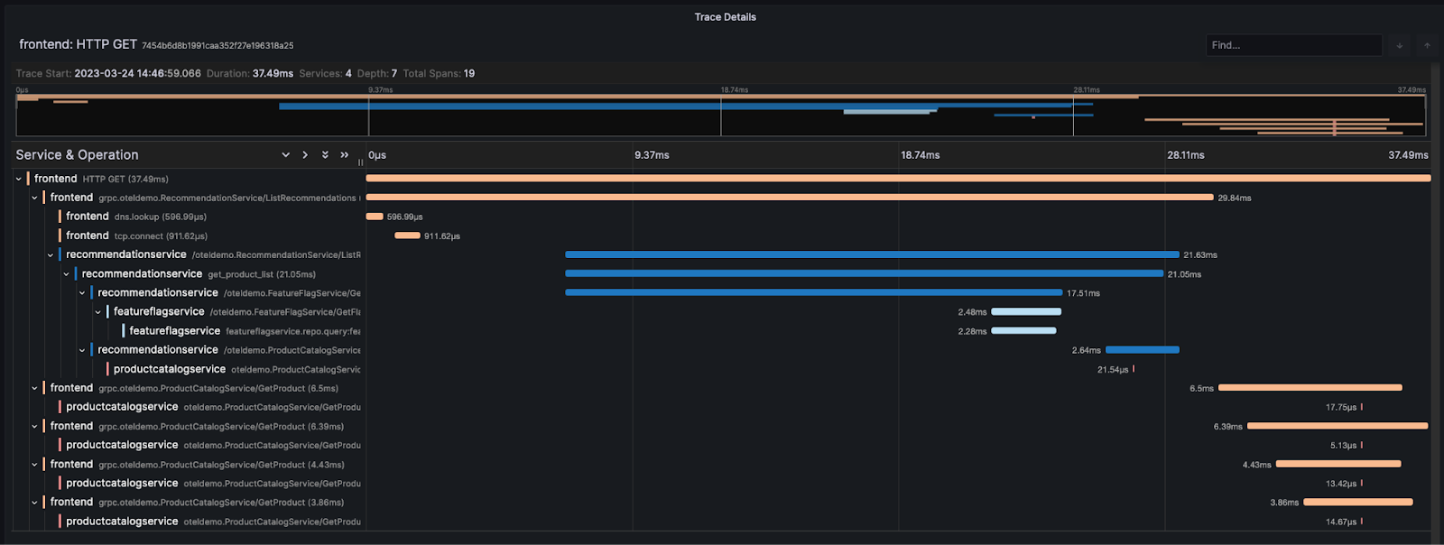
Using variables and data links in Grafana, users can produce complex workflows where visualizations can be filtered interactivity. The following dashboard contains several visualizations:
- A overview of service request volume as a stacked bar
- 99th percentile of latency of each service as a multi-line
- Error rates per service as a bar
- A list of traces aggregated by traceId - the service is here the first in the span chain.
- A Trace Panel that populates when we filter to a specific trace.
This dashboard gives us some basic diagnostic capabilities around errors and performance. The OpenTelemetry demo has existing scenarios where the user can enable specific issues on the service. One of these scenarios involves a memory leak in the recommendation service. Without metrics, we can’t complete the entire issue resolution flow but can identify problematic traces. We show this below:
This dashboard is now packaged with the plugin, and available with the demo.
Using Parameterized Views
The above queries can be quite complex. For example, notice how we are forced to utilize an arrayMap function to ensure the attributes are correctly structured. We could defer this work to a materialized or default column at query time, thus simplifying the query. However, this will still require significant SQL. This can be especially tedious when visualizing a trace in the Explore view.
To simplify query syntax, ClickHouse offers parameterized views. Parametrized views are similar to normal views but can be created with parameters that are not resolved immediately. These views can be used with table functions, which specify the name of the view as the function name and the parameter values as its arguments. This can dramatically reduce the end user's required syntax in ClickHouse. Below we create a view that accepts a trace id and returns the results required for the Trace View. Although support for CTEs in parametized views was recently added, but below we use the simpler query from earlier:
CREATE VIEW trace_view AS
SELECT
TraceId AS traceID,
SpanId AS spanID,
SpanName AS operationName,
ParentSpanId AS parentSpanID,
ServiceName AS serviceName,
Duration / 1000000 AS duration,
Timestamp AS startTime,
arrayMap(key -> map('key', key, 'value', SpanAttributes[key]), mapKeys(SpanAttributes)) AS tags,
arrayMap(key -> map('key', key, 'value', ResourceAttributes[key]), mapKeys(ResourceAttributes)) AS serviceTags
FROM otel_traces
WHERE TraceId = {trace_id:String}To run this view, we simply pass a trace id e.g.,
SELECT *
FROM trace_view(trace_id = '1f12a198ac3dd502d5201ccccad52967')This can significantly reduce the complexity of querying for traces. Below we use the Explore view to query for a specific trace. Notice the need to set the Format value to Trace to cause rendering of the trace:
Parametrized views are best employed for common workloads where users perform common tasks that require ad-hoc analysis, such as inspecting a specific trace.
Compression
One of the benefits of ClickHouse for storing trace data is its high compression. Using the query below, we can see we achieve compression rates of 9x-10x on the trace data generated by this demo. This dataset was generated by running the demo while subjected to 2000 virtual users for 24 hours using the load generator service provided. We have made this dataset available for public use. This can be inserted using the steps here. For hosting this data, we recommend a development service in ClickHouse Cloud (16GB, two cores), which is more than sufficient for a dataset of this size.
SELECT
formatReadableSize(sum(data_compressed_bytes)) AS compressed_size,
formatReadableSize(sum(data_uncompressed_bytes)) AS uncompressed_size,
round(sum(data_uncompressed_bytes) / sum(data_compressed_bytes), 2) AS ratio
FROM system.columns
WHERE table = 'otel_traces'
ORDER BY sum(data_compressed_bytes) DESC
┌─compressed_size─┬─uncompressed_size─┬─ratio─┐
│ 13.68 GiB │ 132.98 GiB │ 9.72 │
└─────────────────┴───────────────────┴───────┘
1 row in set. Elapsed: 0.003 sec.
SELECT
name,
formatReadableSize(sum(data_compressed_bytes)) AS compressed_size,
formatReadableSize(sum(data_uncompressed_bytes)) AS uncompressed_size,
round(sum(data_uncompressed_bytes) / sum(data_compressed_bytes), 2) AS ratio
FROM system.columns
WHERE table = 'otel_traces'
GROUP BY name
ORDER BY sum(data_compressed_bytes) DESC
┌─name───────────────┬─compressed_size─┬─uncompressed_size─┬───ratio─┐
│ ResourceAttributes │ 2.97 GiB │ 78.49 GiB │ 26.43 │
│ TraceId │ 2.75 GiB │ 6.31 GiB │ 2.29 │
│ SpanAttributes │ 1.99 GiB │ 22.90 GiB │ 11.52 │
│ SpanId │ 1.68 GiB │ 3.25 GiB │ 1.94 │
│ ParentSpanId │ 1.35 GiB │ 2.74 GiB │ 2.02 │
│ Events.Timestamp │ 1.02 GiB │ 3.47 GiB │ 3.4 │
│ Timestamp │ 955.77 MiB │ 1.53 GiB │ 1.64 │
│ Duration │ 619.43 MiB │ 1.53 GiB │ 2.53 │
│ Events.Attributes │ 301.09 MiB │ 5.12 GiB │ 17.42 │
│ Links.TraceId │ 36.52 MiB │ 1.60 GiB │ 44.76 │
│ Events.Name │ 22.92 MiB │ 248.91 MiB │ 10.86 │
│ Links.SpanId │ 17.77 MiB │ 34.49 MiB │ 1.94 │
│ HostName │ 8.32 MiB │ 4.56 GiB │ 561.18 │
│ StatusCode │ 1.11 MiB │ 196.80 MiB │ 177.18 │
│ StatusMessage │ 1.09 MiB │ 219.08 MiB │ 201.86 │
│ SpanName │ 538.55 KiB │ 196.82 MiB │ 374.23 │
│ SpanKind │ 529.98 KiB │ 196.80 MiB │ 380.25 │
│ ServiceName │ 529.09 KiB │ 196.81 MiB │ 380.9 │
│ TraceState │ 138.05 KiB │ 195.93 MiB │ 1453.35 │
│ Links.Attributes │ 11.10 KiB │ 16.23 MiB │ 1496.99 │
│ Links.TraceState │ 1.71 KiB │ 2.03 MiB │ 1218.44 │
└────────────────────┴─────────────────┴───────────────────┴─────────┘
20 rows in set. Elapsed: 0.003 sec.We explore schema optimization and how this compression rate can be further improved in a later blog post in this series.
Further work
The current ClickHouse Exporter is in alpha. This state reflects the relative recency of its release and maturity. While we plan to invest in this exporter, we have identified a number of challenges and possible improvements:
-
Schema - The schema contains a number of optimizations that potentially be premature. The use of bloom filters may be unnecessary for some workloads. As shown below, these consume space (around 1% of the total data size).
SELECT formatReadableSize(sum(secondary_indices_compressed_bytes)) AS compressed_size, formatReadableSize(sum(secondary_indices_uncompressed_bytes)) AS uncompressed_size FROM system.parts WHERE (table = 'otel_traces') AND active ┌─compressed_size─┬─uncompressed_size─┐ │ 425.54 MiB │ 1.36 GiB │ └─────────────────┴───────────────────┘We have found the filter on the
TraceIdcolumn to be effective and a worthy addition to the schema. This seems to negate most of the benefit of the materialized view, which adds questionable value for the additional query and maintenance complexity. However, it provides an excellent example of how materialized views can potentially be applied to accelerate queries. We have insufficient evidence to testify to the value of other bloom filters and would recommend users experiment. -
High memory - We have found the OTEL collector to be very memory intensive. In the earlier configuration, we use the batch processor to send data to ClickHouse after 5s or when the batch reaches 100,000 rows. While this optimizes for ClickHouse inserts and adheres to best practices, it can be very memory intensive under high load - especially when collecting logs. This can be mitigated by reducing the flush time and/or batch size. Be aware that this requires tuning as it may cause excessive parts to accumulate in ClickHouse. Alternatively, users may wish to use asynchronous inserts to send data. This will reduce the batch size but is only supported over HTTP in the exporter. To activate, use the
connection_paramsin the exporter config, e.g.,connection_params: async_insert: 1 wait_for_async_insert: 0Note that this will not be as efficient for inserts to ClickHouse.
-
End-to-end delivery - We currently see no support for end-to-end delivery guarantees. i.e., the application SDKs will consider a trace sent once the Collector receives it. If the OTEL Collector crashes, batches currently in memory will be lost. This can be mitigated by reducing the batch size (see above). However, users may also wish to consider alternative architectures involving Kafka (see receiver and exporter) or equivalent persistent queues if higher delivery guarantees are required. We have not explored the recent persistent queues feature, which is in alpha but promises to improve resilience.
-
Scaling - The above deployment only utilizes a single collector. In a high-volume production environment, it is likely users would need to deploy multiple collectors behind a load balancer. The OTEL collector supports this using a Trace Id/Service Name load-balancing exporter. This ensures spans from the same trace are forwarded to the same collector. Note that we have also made no effort to tune agents or measure their resource overhead - something we recommend users research or do before production deployment. We plan to explore these topics in later posts.
-
Sampling - Our current implementation results in all data being stored in ClickHouse. While ClickHouse offers fantastic compression, we appreciate that users will wish to employ sampling techniques. This allows only a subset of traces to be stored, thus reducing hardware requirements. Be aware this complicates scaling. We will address this in a later post.
Conclusion
This blog post shows how traces can easily be collected and stored in ClickHouse using OpenTelemetry. We have forked the OpenTelemetry demo to support ClickHouse, touched on queries and visualization techniques using Grafana, and highlighted some approaches to reducing query complexity and some of the future work for the project. For further reading, we encourage users to explore topics beyond this post, such as how the OTEL collector can be deployed at scale, handling backpressure, and delivery guarantees. We will explore these topics in a later post and add metrics data to our ClickHouse instance before also exploring how schemas can be optimized, and data managed with lifecycle features.