In this article, we explore the world of MLOps and how data in OLAP databases can be modeled and transformed to allow it to act as an efficient feature store for training ML models. While the lessons shared are applicable to a range of OLAP systems, we will use ClickHouse as an example to demonstrate these techniques - for no reason other than we know it well!
The approaches discussed in this blog are used by existing ClickHouse users, who we thank for sharing their techniques, as well as out of the box feature stores.
We focus on using an ClickHouse as a data source, offline store, and transformation engine. These components of a feature store are fundamental to delivering data efficiently and correctly to model training. While most out-of-the-box feature stores provide abstractions, we peel back the layers and describe how data can be modeled efficiently to build and serve features. For users looking to build their own feature store, or just curious as to the techniques existing stores use, read on.
Why ClickHouse?
We have explored what a feature store is in previous blog posts and recommend users are familiar with the concept before diving into this one. In its simplest form, a feature store is a centralized repository for storing and managing data that will be used to train ML models, aiming to improve collaboration and reusability and reduce model iteration time.
As a real-time data warehouse, ClickHouse can fulfill two primary components of a feature store beyond simply providing a datasource.
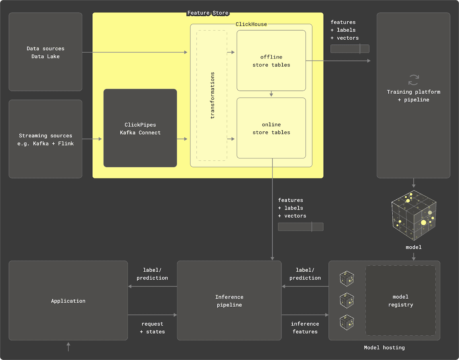
- Transformation Engine: ClickHouse utilizes SQL for declaring data transformations, optimized by its analytical and statistical functions. It supports querying data from various sources, such as Parquet, Postgres, and MySQL, and performs aggregations over petabytes of data. Materialized views allow data transformations at insert time. Additionally, ClickHouse can be used in Python via chDB for transforming large data frames.
- Offline Store: ClickHouse can persist query results through
INSERT INTO SELECTstatements, automatically generating table schemas. It supports efficient data iteration and scaling, with features often represented in tables with timestamps for point-in-time queries. ClickHouse’s sparse indices andASOF LEFT JOINclause facilitate fast filtering and feature selection, optimizing data preparation for training pipelines. This work is parallelized and executed across a cluster, enabling the offline store to scale to petabytes while keeping the feature store lightweight.
In this post, we show how data can be modeled and managed in ClickHouse to perform these roles.
High-level steps
When using ClickHouse as the basis for your offline feature store, we think of the steps to train a model as consisting of the following:
-
Exploration - Familiarize yourself with source data in ClickHouse with SQL queries.
-
Identify the data subset and features - Identify the possible features, their respective entities, and the subset of data needed to produce them. We refer to the subset from this step as the "feature subset."
-
Creating Features - Create the SQL queries required to generate the features.
-
Generating model data - Combine the features appropriately to produce a set of feature vectors, usually achieved using an ASOF JOIN on a common key and timestamp proximity.
-
Generating test and training sets - Split the "feature subset" into a test and training set (and possibly validation).
-
Train model - Train model(s) using the training data, possibly with different algorithms.
-
Model selection & tuning - Evaluate models against the validation set, choose the best model, and fine-tune hyperparameters.
-
Model evaluation - Evaluate the final model against the test set. If performance is sufficient, stop; otherwise, return to 2.
We concern ourselves with steps (1) to (5) as these are ClickHouse-specific. One of the key properties of the above process is that it is highly iterative. Steps (3) and (4) could be loosely referred to as "Feature engineering" and something that typically consumes more time than choosing the model and refining the hyperparameters. Optimizing this process and ensuring ClickHouse is used as efficiently as possible can, therefore, deliver significant time and cost savings.
We explore each of these steps below and propose a flexible approach that optimally leverages ClickHouse features, allowing users to iterate efficiently.
Dataset & Example
For our example, we use the following web analytics dataset, described here. This dataset consists of 100m rows, with an event representing a request to a specific URL. The ability to train machine learning models on web analytics data in ClickHouse is a common use case we see amongst users[1][2].
Due to its size, the following table has been truncated to columns we will use. See here for the full schema.
CREATE TABLE default.web_events
(
`EventTime` DateTime,
`UserID` UInt64,
`URL` String,
`UserAgent` UInt8,
`RefererCategoryID` UInt16,
`URLCategoryID` UInt16,
`FetchTiming` UInt32,
`ClientIP` UInt32,
`IsNotBounce` UInt8,
-- many more columns...
)
ENGINE = MergeTree
PARTITION BY toYYYYMM(EventDate)
ORDER BY (CounterID, EventDate, intHash32(UserID))To illustrate the modeling steps, let's suppose we wish to use this dataset to build a model that predicts whether a user will bounce when a request arrives. If we consider the above source data, this is denoted by the column IsNotBounce. This represents our target class or label.
We aren't going to actually build this model and provide the Python code, rather focusing on the data modeling process. For this reason, our choice of features is illustrative only.
Step 1 - Exploration
Exploring and understanding the source data requires users to become familiar with ClickHouse SQL. We recommend users familiarize themselves with ClickHouse's wide range of analytical functions during this step. Once familiar with the data, we can begin identifying the features for our model and the subset of the data required to produce them.
Step 2 - Features and subsets
To predict whether a visit will bounce, our model will require a training set where each data point contains appropriate features assembled into a feature vector. Typically, these features will be based on a subset of the data.
We've explored the concept of features and feature vectors in other blogs and how they loosely correlate to a column and row of a result set, respectively. Importantly, they need to be available at training and request time.
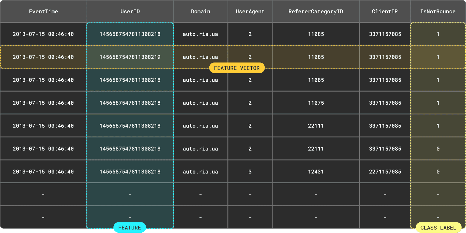
Note we emphasized "result set" above. A feature vector is rarely just a row from a table with the features of a subset of the columns. Often, a complex query must be issued to compute the feature from an aggregation or transformation.
Identifying features
Before identifying features, we should be aware of two of the key properties that will influence our modeling process:
-
Association with entities - Features are typically associated with an
entitywith which they are associated or "keyed". For our problem, the features we think might be useful in making a prediction might be a mixture of user or domain-based. A user-based feature would be request-specific, e.g., the user's age, client IP, or user agent. A domain feature would be associated with the page visited e.g.number of visits per year.Associating features with an instance of an entity requires the entity to have a key or identifier. In our case we need an identifier for the user and a domain value. These are available from the
UserIDandURLcolumns, respectively. The domain can be extracted from the URL using the domain function in ClickHouse, i.e.,domain(URL). -
Dynamic & complex - While certain features remain relatively static, e.g., the user's age, others, such as the client IP, will exhibit changes over time. In such cases, we need to access the feature’s value as it existed at a specific timestamp. This is key for creating point-in-time correct training sets.
While some features will likely be simple, e.g., whether the device is mobile or the client IP, other more complicated features require aggregate statistics, which change over time - and this is where ClickHouse excels!
Example features
For example, suppose we consider the following features to be useful in predicting whether a website visit will bounce. All of our features are associated with a timestamp as they are dynamic and change over time.
- User-agent of the visit - Associated with the user entity and available in the column
UserAgent. - Category of the referrer - (e.g., search engine, social media, direct). A user feature available through the column
RefererCategoryID. - Number of domains visited per hour - at the time the user made the request. Requires a
GROUP BYto compute this user feature. - Number of unique IPs visiting the domain per hour - Domain feature requiring a
GROUP BY. - Category of the page - User feature available through the column
URLCategoryID. - Average request time for the domain per hour - Requires a
GROUP BYto compute this from theFetchTimingcolumn.
These features might not be ideal and illustrative only. Linking many of these features to the user entity is somewhat simplistic. For instance, some features would be more accurately associated with the request or session entity.
Feature subsets
Once we have an idea of the features we will use, we can identify the required subset of the data needed to build them. This step is optional as sometimes users wish to use the whole data, or the data isn't large and complex enough to warrant this step.
When applied, we often see users creating tables for their model data - we refer to these as the "feature subset". These consist of:
- The entity values for each feature vector.
- A timestamp of the event if it exists.
- Class label.
- The columns needed to produce the planned features. Users may wish to add other columns that they consider useful in future iterations.
This approach provides several advantages:
-
Allows the data to be ordered and optimized for future accesses. Typically, the model data will be read and filtered differently than the source data. These tables can also generate features faster than the source data when producing a final training set.
-
A subset or transformed set of data may be required for the model. Identifying, filtering, and transforming this subset may be an expensive query. By inserting the data into an intermediate model table, this query only has to be executed once. Subsequent feature generation and model training runs can thus obtain the data efficiently from this table.
We can use this step to de-duplicate any data. While the raw data might not contain duplicates, the resulting subset may if we extract a subset of the columns for features.
Suppose for our model we create an intermediate table predict_bounce_subset. This table needs the EventTime, the label IsNotBounce, and the entity keys Domain and UserID. Additionally, we include the simple feature columns UserAgent, RefererCategoryID , and URLCategoryID, as well as those needed to produce our aggregate features - FetchTiming and ClientIP.
CREATE TABLE predict_bounce_subset
(
EventTime DateTime64,
UserID UInt64,
Domain String,
UserAgent UInt8,
RefererCategoryID UInt16,
URLCategoryID UInt16,
FetchTiming UInt32,
ClientIP UInt32,
IsNotBounce UInt8
)
ENGINE = ReplacingMergeTree
ORDER BY (EventTime, Domain, UserID, UserAgent, RefererCategoryID, URLCategoryID, FetchTiming, ClientIP, IsNotBounce)
PRIMARY KEY (EventTime, Domain, UserID)We use a ReplacingMergeTree as our table engine. This engine de-duplicates rows that have the same values in the ordering key columns. This is performed asynchronously in the background at merge tree, although we can ensure we don't receive duplicates at query time using the FINAL modifier. This approach to deduplication tends to be more resource efficient than the alternative in this scenario - using a GROUP BY of the columns we wish to de-duplicate data by at insert time below. Above, we assume all columns should be used to identify unique rows. It is possible to have events with the same EventTime, UserID, Domain, e.g. multiple requests made when visiting a domain with different FetchTiming values.
Further details on the ReplacingMergeTree can be found here.
As an optimization, we only load a subset of the ordering keys into the primary key (held in memory) via the
PRIMARY KEYclause. By default, all columns in theORDER BYare loaded. In this case, we will likely only want to query by theEventTime,Domain, andUserID.
Suppose we wish to only train our bounce prediction model on events not associated with bots - identified by Robotness=0. We also will require a Domain and UserID value.
We can populate our predict_bounce_subset table using an INSERT INTO SELECT, reading the rows from web_events and applying filters that reduce our data size to 42m rows.
INSERT INTO predict_bounce_subset SELECT
EventTime,
UserID,
domain(URL) AS Domain,
UserAgent,
RefererCategoryID,
URLCategoryID,
FetchTiming,
ClientIP,
IsNotBounce
FROM web_events
WHERE Robotness = 0 AND Domain != '' AND UserID != 0
0 rows in set. Elapsed: 7.886 sec. Processed 99.98 million rows, 12.62 GB (12.68 million rows/s., 1.60 GB/s.)
SELECT formatReadableQuantity(count()) AS count
FROM predict_bounce_subset FINAL
┌─count─────────┐
│ 42.89 million │
└───────────────┘
1 row in set. Elapsed: 0.003 sec.Note the use of the
FINALclause above to ensure we only count unique rows.
Updating feature subsets
While some subsets of data are static, others will be subject to change as new events arrive in the source table. Often, users, therefore, need to keep subsets up-to-date. While this can be achieved with scheduled queries that rebuild the tables (e.g., using dbt), ClickHouse (incremental) Materialized views can be used to maintain these.
Materialized views allow users to shift the cost of computation from query time to insert time. A ClickHouse materialized view is just a trigger that runs a query on blocks of data as they are inserted into a table e.g., the web_events table. The results of this query are then inserted into a second "target" table - the subset table in our case. Should more rows be inserted, results will again be sent to the target table. This merged result is the equivalent of running the query over all of the original data.
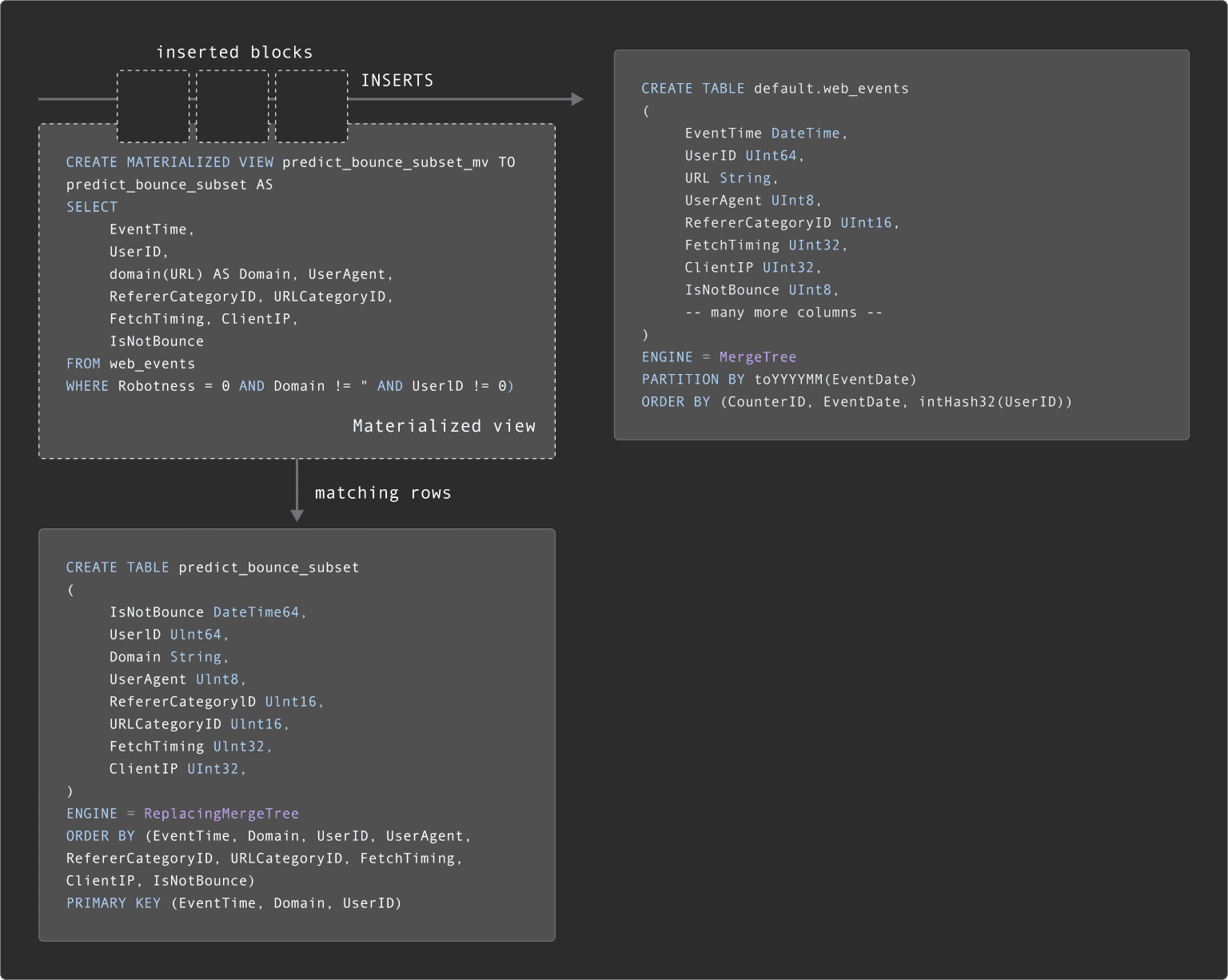
A materialized which maintains our predict_bounce_subset is shown below:
CREATE MATERIALIZED VIEW predict_bounce_subset_mv TO predict_bounce_subset AS
SELECT
EventTime,
UserID,
domain(URL) AS Domain,
UserAgent,
RefererCategoryID,
URLCategoryID,
FetchTiming,
ClientIP,
IsNotBounce
FROM web_events
WHERE Robotness = 0 AND Domain != '' AND UserID != 0This is a simple example, and we recommend that users learn more about the power of materialized views here. For the subsequent steps, we assume we will use the model table predict_bounce_subset.
Step 3 - Creating Features
For model training, we'll need to assemble our planned features into a set of feature vectors with the label IsNotBounce i.e.

Note how we assemble our feature vector from features from multiple entities. In many cases we are looking for the feature value at the closest point in time from another entity.
An experienced SQL developer familiar with ClickHouse could probably formulate a query that produced the above feature vector. While possible, this will invariably not only be a complex and computationally expensive query - especially over larger datasets of billions of rows.
Furthermore as noted, our feature vectors are dynamic and potentially consist of any number of combinations of different features during different training iterations. Additionally, ideally different engineers and data scientists would be using the same definition of a feature as well as writing the queries as optimally as possible.
Given the above demands, it makes sense to materialize our features into tables writing the results of the query into a table using INSERT INTO SELECT. This effectively means we perform the feature generation once, writing the results to a table from which they can be efficiently read and reused when iterating. This also allows us to declare the feature query once, optimally, and share the results with other engineers and scientists.
For now, we omit how users might wish to declare, version control, and share their feature definitions. SQL is, after all, code. There are several solutions to this problem, some of which solve different challenges - see "Build or Adopt".
Feature tables
A feature table contains instances of a feature associated with an entity and, optionally, a timestamp. We have seen our users employ two table models for features - either creating a table per feature or per entity. Each approach has its respective pros and cons we explore below. Both of these allow re-usability of the features though, with the advantage they ensure the data is compressed well.
You don't need to create a feature table for every feature. Some can be consumed from the model table as-is, in cases where they are represented by a column value.
Feature tables (per feature)
With a table per feature, the table name denotes the feature itself. The primary advantage of this approach is it potentially simplifies later joins. Additionally, it means users can use materialized views to maintain these tables as the source data changes - see "Updating".
The disadvantage of this approach is it doesn't scale as well as the "per event". Users with thousands of features will have thousands of tables. While possibly manageable, creating materialized views to maintain each of these is not viable.
As an example, consider the table responsible for storing the domain feature "number of unique IPs for each domain".
CREATE TABLE number_unique_ips_per_hour
(
Domain String,
EventTime DateTime64,
Value Int64
)
ENGINE = MergeTree
ORDER BY (Domain, EventTime)We have chosen the ORDER BY key to optimize both compression and future reads. We can populate our feature table using a simple INSERT INTO SELECT with an aggregation to compute our feature.
INSERT INTO number_unique_ips_per_hour SELECT
Domain,
toStartOfHour(EventTime) AS EventTime,
uniqExact(ClientIP) AS Value
FROM predict_bounce_subset FINAL
GROUP BY
Domain,
EventTime
0 rows in set. Elapsed: 0.777 sec. Processed 43.80 million rows, 1.49 GB (56.39 million rows/s., 1.92 GB/s.)
SELECT count()
FROM number_unique_ips_per_hour
┌─count()─┐
│ 613382 │
└─────────┘We choose to use Domain and Value as the column name for entity and feature value. This makes our future queries a little simpler. Users may wish to use a generic table structure for all features, with an Entity and Value column.
CREATE TABLE <feature_name>
(
Entity Variant(UInt64, Int64, String),
EventTime DateTime64,
Value Variant(UInt64, Int64, Float64)
)
ENGINE = MergeTree
ORDER BY (Entity, EventTime)This requires the use of the Variant type. This type allows a column to support a union of other data types e.g. Variant(String, Float64, Int64) means that each row of this type has a value of either type String, Float64 Int64 or none of them (NULL value).
This feature is currently experimental and optional for the above approach but required for the "Per entity" approach described below.
Feature tables (per entity)
In a per entity approach we use the same table for all features which are associated with the same entity. In this case, we use a column, FeatureId below, to denote the name of the feature.
The advantage of this approach is its scalability. A single table can easily hold thousands of features.
The principal disadvantage is that currently materialized views are not supported by this approach.
Note we are forced to use the new Variant type in the below example for the domain features. While this table supports UInt64, Int64, and Float64 feature values, it could potentially support more.
-- domain Features
SET allow_experimental_variant_type=1
CREATE TABLE domain_features
(
Domain String,
FeatureId String,
EventTime DateTime,
Value Variant(UInt64, Int64, Float64)
)
ENGINE = MergeTree
ORDER BY (FeatureId, Domain, EventTime)This table's ORDER BY is optimized for filtering by a specific FeatureId and Domain - the typical access pattern we will see later.
To populate our "number of unique IPs for each domain" feature into this table, we need a similar query to that used earlier:
INSERT INTO domain_features SELECT
Domain,
'number_unique_ips_per_hour' AS FeatureId,
toStartOfHour(EventTime) AS EventTime,
uniqExact(ClientIP) AS Value
FROM predict_bounce_subset FINAL
GROUP BY
Domain,
EventTime
0 rows in set. Elapsed: 0.573 sec. Processed 43.80 million rows, 1.49 GB (76.40 million rows/s., 2.60 GB/s.)
SELECT count()
FROM domain_features
┌─count()─┐
│ 613382 │
└─────────┘Users new to ClickHouse may wonder if the "per feature" approach allows faster retrieval of features than the "per entity" approach. Due to the use of ordering keys and ClickHouse sparse indices, there should be no difference here.
Updating feature tables
While some features are static, we often want to ensure they are updated as the source data or subsets change. As described for "Updating subsets", we can achieve this with Materialized views.
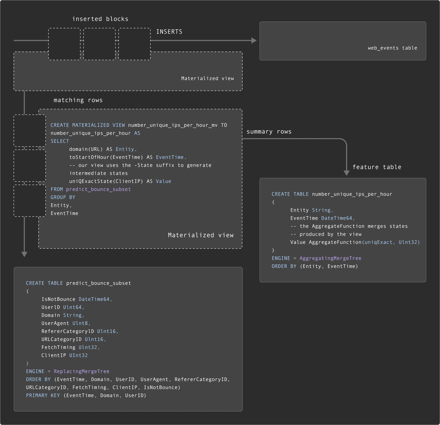
In the case of feature tables, our materialized views are typically more complex as the results are often the results of aggregation and not just simple transformations and filtering. As a result, the query executed by the materialized view will produce partial aggregation states. These partial aggregation states represent the intermediate state of the aggregation, which the target feature table can merge together. This requires our feature table to use the AggregatingMergeTree with appropriate AggregateFunction types.
We provide an example below for a "per feature" table number_unique_ips_per_hour.
CREATE TABLE number_unique_ips_per_hour
(
Entity String,
EventTime DateTime64,
-- the AggregateFunction merges states produced by the view
Value AggregateFunction(uniqExact, UInt32)
)
ENGINE = AggregatingMergeTree
ORDER BY (Entity, EventTime)
CREATE MATERIALIZED VIEW number_unique_ips_per_hour_mv TO number_unique_ips_per_hour AS
SELECT
domain(URL) AS Entity,
toStartOfHour(EventTime) AS EventTime,
-- our view uses the -State suffix to generate intermediate states
uniqExactState(ClientIP) AS Value
FROM predict_bounce_subset
GROUP BY
Entity,
EventTimeAs new rows are inserted into the predict_bounce_subset table, our number_unique_ips_per_hour feature table will be updated.
When querying number_unique_ips_per_hour, we must either use the FINAL clause or GROUP BY Entity, EventTime to ensure aggregation states are merged along with the -Merge variant of the aggregation function (in this case, uniqExact). As shown this below, this alters the query used to fetch entities - see here for further details.
-- Select entities for a single domain
SELECT
EventTime,
Entity,
uniqExactMerge(Value) AS Value
FROM number_unique_ips_per_hour
WHERE Entity = 'smeshariki.ru'
GROUP BY
Entity,
EventTime
ORDER BY EventTime DESC LIMIT 5
┌───────────────EventTime─┬─Entity────────┬─Value─┐
│ 2013-07-31 23:00:00.000 │ smeshariki.ru │ 3810 │
│ 2013-07-31 22:00:00.000 │ smeshariki.ru │ 3895 │
│ 2013-07-31 21:00:00.000 │ smeshariki.ru │ 4053 │
│ 2013-07-31 20:00:00.000 │ smeshariki.ru │ 3893 │
│ 2013-07-31 19:00:00.000 │ smeshariki.ru │ 3926 │
└─────────────────────────┴───────────────┴───────┘
5 rows in set. Elapsed: 0.491 sec. Processed 8.19 thousand rows, 1.28 MB (16.67 thousand rows/s., 2.61 MB/s.)
Peak memory usage: 235.93 MiB.While a little more complex, intermediate aggregation states allow us to use the above table to generate features for different times. For example, we could compute the number of unique IPs per domain per day from the above table using this query, something we couldn't do with our original feature table.
Users may notice that our subset table predict_bounce_subset is being updated with a materialized view already, which in turn has Materialized views attached to it. As shown below, this means our Materialized views are effectively "chained". For more examples of chaining Materialized views, see here.
Updating per entity feature tables
The above "per feature" approach to modeling means a materialized view per feature table (a materialized view can send results to only one table). In larger use cases, this becomes a constraint on scaling - materialized views incur an insert time overhead, and we don't recommend more than 10 on a single table.
A "per entity" feature table model reduces the number of feature tables. In order to encapsulate multiple queries for different features would require us to use Variant type with AggregateFunction types. This is currently not supported.
As an alternative, users can use Refreshable Materialized Views (currently experimental). Unlike ClickHouse's incremental materialized views, these views periodically execute the view query over the entire dataset, storing the results in a target table whose contents are atomically replaced.

Users can use this capability to periodically update feature tables on a schedule. We provide an example of this below, where the "number of unique IPs for each domain" is updated every 10 minutes.
--enable experimental feature
SET allow_experimental_refreshable_materialized_view = 1
CREATE MATERIALIZED VIEW domain_features_mv REFRESH EVERY 10 MINUTES TO domain_features AS
SELECT
Domain,
'number_unique_ips_per_hour' AS FeatureId,
toStartOfHour(EventTime) AS EventTime,
uniqExact(ClientIP) AS Value
FROM predict_bounce_subset
GROUP BY
Domain,
EventTimeFurther details on Refreshable Materialized views can be found here.
Step 4 - Generating model data
With our features created, we can begin the process of combining these into our model data - which will form the basis of our training, validation and test set.
The rows in this table will form the basis of our model, with each row corresponding to a feature vector. To generate this, we need to join our features. Some of these features will come from feature tables, others directly from our "features subset" table i.e. predict_bounce_subset above.
As the feature subset table contains our events with the label, timestamp, and entity keys, it makes sense for this to form the base table of the join (left-hand side). This is also likely to be the largest table, making it a sensible choice for the left-hand side of the join.
Features will be joined to this table based on two criteria:
- the closest timestamp (
EventTime) for each feature to the row in the feature subset table (predict_bounce_subset). - the corresponding entity column for the feature table, e.g.,
UserIDorDomain.
To join based on this equi join AND the closest time requires an ASOF JOIN.
We will send the results of this join to a table, using an INSERT INTO, which we refer to as the "model table". This will be used to produce future training, validation and test sets.
Before exploring the join, we declare our "model table" predict_bounce.
CREATE TABLE predict_bounce_model (
Row UInt64,
EventTime DateTime64,
UserID UInt64,
Domain String,
UserAgent UInt8,
RefererCategoryID UInt16,
URLCategoryID UInt16,
DomainsVisitedPerHour UInt32 COMMENT 'Number of domains visited in last hour by the user',
UniqueIPsPerHour UInt32 COMMENT 'Number of unique ips visiting the domain per hour',
AverageRequestTime Float32 COMMENT 'Average request time for the domain per hour',
IsNotBounce UInt8,
) ENGINE = MergeTree
ORDER BY (Row, EventTime)The Row column here will contain a unique entry for each row in the dataset. We make this part of our ORDER BY and exploit it later to produce training and test sets efficiently.
Joining and aligning features
To join and align features based on the entity key and timestamp, we can use the ASOF. How we construct our JOIN depends on several factors whether we are using "per feature" or "per entity" feature tables.
Let's assume we are using "per feature" tables and have the following available:
number_unique_ips_per_hour- containing the number of unique ips visiting each domain per hour. Example above.domains_visited_per_hour- Number of domains visited in last hour by each user. Generated using the queries here.average_request_time- Average request time for each domain per hour. Generated using the queries here.
Our JOIN here is quite straightforward:
INSERT INTO predict_bounce_model SELECT
rand() AS Row,
mt.EventTime AS EventTime,
mt.UserID AS UserID,
mt.Domain AS Domain,
mt.UserAgent,
mt.RefererCategoryID,
mt.URLCategoryID,
dv.Value AS DomainsVisitedPerHour,
uips.Value AS UniqueIPsPerHour,
art.Value AS AverageRequestTime,
mt.IsNotBounce
FROM predict_bounce_subset AS mt FINAL
ASOF JOIN domains_visited_per_hour AS dv ON (mt.UserID = dv.UserID) AND (mt.EventTime >= dv.EventTime)
ASOF JOIN number_unique_ips_per_hour AS uips ON (mt.Domain = uips.Domain) AND (mt.EventTime >= uips.EventTime)
ASOF JOIN average_request_time AS art ON (mt.Domain = art.Domain) AND (mt.EventTime >= art.EventTime)
0 rows in set. Elapsed: 13.440 sec. Processed 89.38 million rows, 3.10 GB (6.65 million rows/s., 230.36 MB/s.)
Peak memory usage: 2.94 GiB.
SELECT * FROM predict_bounce_model LIMIT 1 FORMAT Vertical
Row 1:
──────
Row: 57
EventTime: 2013-07-10 06:11:39.000
UserID: 1993141920794806602
Domain: smeshariki.ru
UserAgent: 7
RefererCategoryID: 16000
URLCategoryID: 9911
DomainsVisitedPerHour: 1
UniqueIPsPerHour: 16479
AverageRequestTime: 182.69382
IsNotBounce: 0While similar, this join becomes a little more complex (and costly) if using "per entity" feature tables. Assuming we have the feature tables domain_features and user_features populated with these queries.
INSERT INTO predict_bounce_model SELECT
rand() AS Row,
mt.EventTime AS EventTime,
mt.UserID AS UserID,
mt.Domain AS Domain,
mt.UserAgent,
mt.RefererCategoryID,
mt.URLCategoryID,
DomainsVisitedPerHour,
UniqueIPsPerHour,
AverageRequestTime,
mt.IsNotBounce
FROM predict_bounce_subset AS mt FINAL
ASOF LEFT JOIN (
SELECT Domain, EventTime, Value.UInt64 AS UniqueIPsPerHour
FROM domain_features
WHERE FeatureId = 'number_unique_ips_per_hour'
) AS df ON (mt.Domain = df.Domain) AND (mt.EventTime >= df.EventTime)
ASOF LEFT JOIN (
SELECT Domain, EventTime, Value.Float64 AS AverageRequestTime
FROM domain_features
WHERE FeatureId = 'average_request_time'
) AS art ON (mt.Domain = art.Domain) AND (mt.EventTime >= art.EventTime)
ASOF LEFT JOIN (
SELECT UserID, EventTime, Value.UInt64 AS DomainsVisitedPerHour
FROM user_features
WHERE FeatureId = 'domains_visited_per_hour'
) AS dv ON (mt.UserID = dv.UserID) AND (mt.EventTime >= dv.EventTime)
0 rows in set. Elapsed: 12.528 sec. Processed 58.65 million rows, 3.08 GB (4.68 million rows/s., 245.66 MB/s.)
Peak memory usage: 3.16 GiB.The above joins use a hash join. 24.7 added support for the
full_sorting_mergealgorithm forASOF JOIN. This algorithm can exploit the sort order of the tables being joined, thus avoiding a sorting phase prior to joining. The joined tables can be filtered by each other's join keys prior to any sort and merge operations in order to minimize the amount of processed data. This will allow the above queries to be as fast while consuming fewer resources.
Step 5 - Generating test and training sets
With model data generated, we can produce training, validation, and test sets as required. Each of these will consist of different percentages of the data e.g. 80, 10, 10. Across query executions these need to be consistent results - we can't allow test data to seep into training and vise versa. Furthermore, the result sets need to be stable - some algorithms can be influenced by the order in which the data is delivered, delivering different results.
To achieve consistency and stability of results while also ensuring queries return rows quickly, we can exploit the Row and EventTime columns.
Suppose we wish to obtain 80% of the data for our training in order of EventTime. This can be obtained from our predict_bounce_model table with a simple query that performs a mod 100 on the Row column:
SELECT * EXCEPT Row
FROM predict_bounce_model
WHERE (Row % 100) < 80
ORDER BY EventTime, Row ASCWe can confirm these rows deliver stable results with a few simple queries:
SELECT
groupBitXor(sub) AS hash,
count() AS count
FROM
(
SELECT sipHash64(concat(*)) AS sub
FROM predict_bounce_model
WHERE (Row % 100) < 80
ORDER BY
EventTime ASC,
Row ASC
)
┌─────────────────hash─┬────count─┐
│ 14452214628073740040 │ 34315802 │
└──────────────────────┴──────────┘
1 row in set. Elapsed: 8.346 sec. Processed 42.89 million rows, 2.74 GB (5.14 million rows/s., 328.29 MB/s.)
Peak memory usage: 10.29 GiB.
--repeat query, omitted for brevity
┌─────────────────hash─┬────count─┐
│ 14452214628073740040 │ 34315802 │
└──────────────────────┴──────────┘Similarly, a training set and validation set could be obtained with the following, each constituting 10% of the data:
-- validation
SELECT * EXCEPT Row
FROM predict_bounce_model
WHERE (Row % 100) BETWEEN 80 AND 89
ORDER BY EventTime, Row ASC
-- test
SELECT * EXCEPT Row
FROM predict_bounce_model
WHERE (Row % 100) BETWEEN 90 AND 100
ORDER BY EventTime, Row ASCThe exact approach here users use may depend on how they want to separate their training and test set. For our model, it may be better to use all data before a fixed point in time for training, with the test set using all rows after this. Above, our training and test sample data contain data from the full period. This may cause leakage of some information between the two sets e.g. events from the same page visit. We overlook this for the purposes of an example. We recommend adjusting the ordering key on your model table based on how you intend to consume rows - see here for recommendations on selecting an ordering key.
Build vs Adopt
The process described involves multiple queries and complex procedures. When building an offline feature store with ClickHouse, users typically take one of the following approaches:
-
Build Their Own Feature Store: This is the most advanced and complex approach, allowing users to optimize processes and schemas for their specific data. It's often adopted by companies where the feature store is crucial to their business and involves large data volumes, such as in ad-tech.
-
Dbt + Airflow: Dbt is popular for managing data transformations and handling complex queries and data modeling. When combined with Airflow, a powerful workflow orchestration tool, users can automate and schedule the above processes. This approach offers modular and maintainable workflows, balancing custom solutions with existing tools to handle large data volumes and complex queries without a fully custom-built feature store or the workflows imposed by an existing solution.
-
Adopt a Feature Store with ClickHouse: Feature stores like Featureform integrate ClickHouse for data storage, transformation, and serving offline features. These stores manage processes, version features, and enforce governance and compliance rules, reducing data engineering complexity for data scientists. Adopting these technologies depends on how well the abstractions and workflows fit the use case.
 Credit: Featureform Feature Store
ClickHouse at inference time
This blog post discusses using ClickHouse as an offline store for generating features for model training. Once trained, a model can be deployed for predictions, requiring real-time data like user ID and domain. Precomputed features, such as "domains visited in the last hour," are necessary for predictions but are too costly to compute during inference. These features need to be served based on the most recent data version, especially for real-time predictions.
ClickHouse, as a real-time analytics database, can handle highly concurrent queries with low latency and high write workloads, thanks to its log-structured merge tree. This makes it suitable for serving features in an online store. Features from the offline store can be materialized to new tables in the same ClickHouse cluster or a different instance using existing capabilities. Further details on this process will be covered in a later post.
Conclusion
This blog has outlined common data modeling approaches for using ClickHouse as an offline feature store and transformation engine. While not exhaustive, these approaches provide a starting point and align with techniques used in feature stores like Featureform, which integrates with ClickHouse. We welcome contributions and ideas for improvement. If you're using ClickHouse as a feature store, let us know!
Learn how to model machine learning data in ClickHouse to accelerate your pipelines and enable the fast building of features over potentially billions of rows.
Get started with ClickHouse Cloud today and receive $300 in credits. At the end of your 30-day trial, continue with a pay-as-you-go plan, or contact us to learn more about our volume-based discounts. Visit our pricing page for details.