Get started with ClickHouse Cloud today and receive $300 in credits. To learn more about our volume-based discounts, contact us or visit our pricing page.

This blog post is part of a series:
- ClickHouse Joins Under the Hood - Hash Join, Parallel Hash Join, Grace Hash Join
- ClickHouse Joins Under the Hood - Full Sorting Merge Join, Partial Merge Join
- ClickHouse Joins Under the Hood - Direct Join
- Choosing the Right Join Algorithm
ClickHouse is an open-source column oriented DBMS, built and optimized for use cases requiring super-low latency analytical queries over large amounts of data. To achieve the best possible performance for analytical applications, it is typical to combine tables in a process known as data denormalization. Flattened tables help minimize query latency by avoiding joins, at the cost of incremental ETL complexity, typically acceptable in return for sub-second queries.
However, we recognize that for some workloads, for instance, those coming from more traditional data warehouses, denormalizing data isn’t always practical, and sometimes part of the source data for analytical queries needs to remain normalized. These normalized tables take less storage and provide flexibility with data combinations, but they require joins at query time for certain types of analysis.
Fortunately, contrary to some misconceptions, joins are fully supported in ClickHouse! In addition to supporting all standard SQL JOIN types, ClickHouse provides additional JOIN types useful for analytical workloads and for time-series analysis. ClickHouse allows you to choose between 6 different algorithms (that we will explore in detail in the next part of this blog series) for the join execution, or allow the query planner to adaptively choose and dynamically change the algorithm at runtime, depending on resource availability and usage.
You can achieve good performance even for joins over large tables in ClickHouse, but this use case in particular currently requires users to carefully select and tune join algorithms for their query workloads. While we expect this also to become more automated and heuristics-driven over time, this blog series provides a deep understanding of the internals of join execution in ClickHouse, so you can optimize joins for common queries used by your applications.
For this post, we will use a normalized relational database example schema in order to demonstrate the different join types available in ClickHouse. In the next posts, we will look deeply under the hood of the 6 different join algorithms that are available in ClickHouse. We will explore how ClickHouse integrates these join algorithms to its query pipeline in order to execute the join types as fast as possible. A future part will cover distributed joins.
Test Data and Resources #
We use Venn diagrams and example queries, on a a normalized IMDB dataset originating from the relational dataset repository, to explain the available join types in ClickHouse.
Instructions for creating and loading the tables are here. The dataset is also available in our playground for users wanting to reproduce queries.
We are going to use 4 tables from our example dataset:

The data in that 4 tables represent movies. A movie can have one or many genres. The roles in a movie are played by actors. The arrows in the diagram above represent foreign-to-primary-key-relationships. e.g. the movie_id column of a row in the genres table contains the id value from a row in the movies table.
There is a many-to-many relationship between movies and actors. This many-to-many relationship is normalized into two one-to-many relationships by using the roles table. Each row in the roles table contains the values of the id columns of the movies table and the actors table.
Join types supported in ClickHouse #
INNER JOIN #

The INNER JOIN returns, for each pair of rows matching on join keys, the column values of the row from the left table, combined with the column values of the row from the right table. If a row has more than one match, then all matches are returned (meaning that the cartesian product is produced for rows with matching join keys).
This query finds the genre(s) for each movie by joining the movies table with the genres table:
SELECT m.name AS name, g.genre AS genre FROM movies AS m INNER JOIN genres AS g ON m.id = g.movie_id ORDER BY m.year DESC, m.name ASC, g.genre ASC LIMIT 10; ┌─name───────────────────────────────────┬─genre─────┐ │ Harry Potter and the Half-Blood Prince │ Action │ │ Harry Potter and the Half-Blood Prince │ Adventure │ │ Harry Potter and the Half-Blood Prince │ Family │ │ Harry Potter and the Half-Blood Prince │ Fantasy │ │ Harry Potter and the Half-Blood Prince │ Thriller │ │ DragonBall Z │ Action │ │ DragonBall Z │ Adventure │ │ DragonBall Z │ Comedy │ │ DragonBall Z │ Fantasy │ │ DragonBall Z │ Sci-Fi │ └────────────────────────────────────────┴───────────┘ 10 rows in set. Elapsed: 0.126 sec. Processed 783.39 thousand rows, 21.50 MB (6.24 million rows/s., 171.26 MB/s.)✎
Note that the INNER keyword can be omitted.
The behavior of the INNER JOIN can be extended or changed, by using one of the following other join types.
(LEFT / RIGHT / FULL) OUTER JOIN #

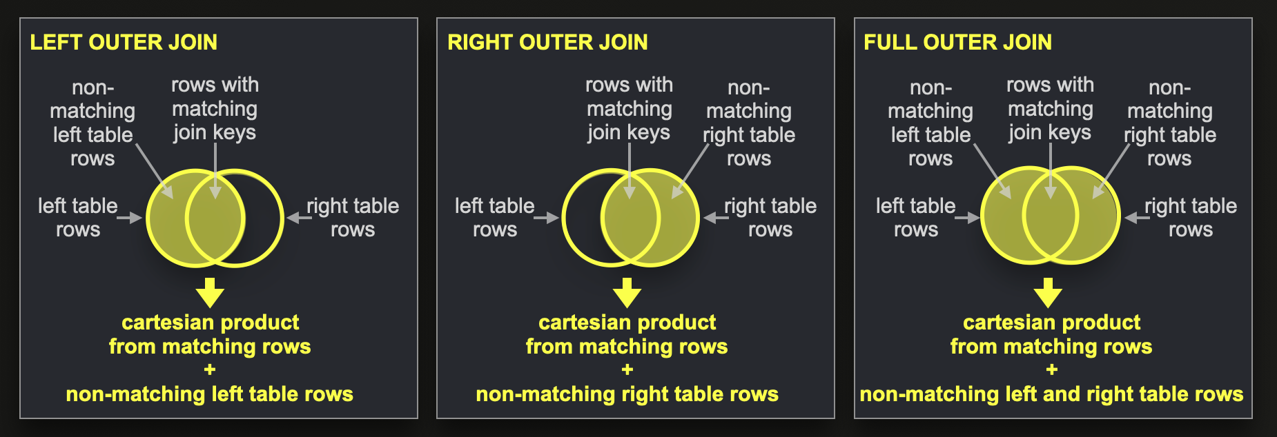
The LEFT OUTER JOIN behaves like INNER JOIN; plus, for non-matching left table rows, ClickHouse returns default values for the right table’s columns.
A RIGHT OUTER JOIN query is similar and also returns values from non-matching rows from the right table together with default values for the columns of the left table.
A FULL OUTER JOIN query combines the LEFT and RIGHT OUTER JOIN and returns values from non-matching rows from the left and the right table, together with default values for the columns of the right and left table, respectively.
Note that ClickHouse can be configured to return NULLs instead of default values (however, for performance reasons, that is less recommended).
This query finds all movies that have no genre by querying for all rows from the movies table that don’t have matches in the genres table, and therefore get (at query time) the default value 0 for the movie_id column:
SELECT m.name FROM movies AS m LEFT JOIN genres AS g ON m.id = g.movie_id WHERE g.movie_id = 0 ORDER BY m.year DESC, m.name ASC LIMIT 10; ┌─name──────────────────────────────────────┐ │ """Pacific War, The""" │ │ """Turin 2006: XX Olympic Winter Games""" │ │ Arthur, the Movie │ │ Bridge to Terabithia │ │ Mars in Aries │ │ Master of Space and Time │ │ Ninth Life of Louis Drax, The │ │ Paradox │ │ Ratatouille │ │ """American Dad""" │ └───────────────────────────────────────────┘ 10 rows in set. Elapsed: 0.092 sec. Processed 783.39 thousand rows, 15.42 MB (8.49 million rows/s., 167.10 MB/s.)✎
Note that the OUTER keyword can be omitted.
CROSS JOIN #

The CROSS JOIN produces the full cartesian product of the two tables without considering join keys. Each row from the left table is combined with each row from the right table.
The following query, therefore, is combing each row from the movies table with each row from the genres table:
SELECT m.name, m.id, g.movie_id, g.genre FROM movies AS m CROSS JOIN genres AS g LIMIT 10; ┌─name─┬─id─┬─movie_id─┬─genre───────┐ │ #28 │ 0 │ 1 │ Documentary │ │ #28 │ 0 │ 1 │ Short │ │ #28 │ 0 │ 2 │ Comedy │ │ #28 │ 0 │ 2 │ Crime │ │ #28 │ 0 │ 5 │ Western │ │ #28 │ 0 │ 6 │ Comedy │ │ #28 │ 0 │ 6 │ Family │ │ #28 │ 0 │ 8 │ Animation │ │ #28 │ 0 │ 8 │ Comedy │ │ #28 │ 0 │ 8 │ Short │ └──────┴────┴──────────┴─────────────┘ 10 rows in set. Elapsed: 0.024 sec. Processed 477.04 thousand rows, 10.22 MB (20.13 million rows/s., 431.36 MB/s.)✎
While the previous example query alone didn’t make much sense, it can be extended with a WHERE clause for associating matching rows to replicate INNER join behavior for finding the genre(s) for each movie:
SELECT m.name AS name, g.genre AS genre FROM movies AS m CROSS JOIN genres AS g WHERE m.id = g.movie_id ORDER BY m.year DESC, m.name ASC, g.genre ASC LIMIT 10; ┌─name───────────────────────────────────┬─genre─────┐ │ Harry Potter and the Half-Blood Prince │ Action │ │ Harry Potter and the Half-Blood Prince │ Adventure │ │ Harry Potter and the Half-Blood Prince │ Family │ │ Harry Potter and the Half-Blood Prince │ Fantasy │ │ Harry Potter and the Half-Blood Prince │ Thriller │ │ DragonBall Z │ Action │ │ DragonBall Z │ Adventure │ │ DragonBall Z │ Comedy │ │ DragonBall Z │ Fantasy │ │ DragonBall Z │ Sci-Fi │ └────────────────────────────────────────┴───────────┘ 10 rows in set. Elapsed: 0.150 sec. Processed 783.39 thousand rows, 21.50 MB (5.23 million rows/s., 143.55 MB/s.)✎
An alternative syntax for CROSS JOIN specifies multiple tables in the FROM clause separated by commas.
ClickHouse is rewriting a CROSS JOIN to an INNER JOIN if there are joining expressions in the WHERE section of the query.
We can check that for the example query via EXPLAIN SYNTAX (that returns the syntactically optimized version into which a query gets rewritten before being executed):
EXPLAIN SYNTAX SELECT m.name AS name, g.genre AS genre FROM movies AS m CROSS JOIN genres AS g WHERE m.id = g.movie_id ORDER BY m.year DESC, m.name ASC, g.genre ASC LIMIT 10; ┌─explain─────────────────────────────────────┐ │ SELECT │ │ name AS name, │ │ genre AS genre │ │ FROM movies AS m │ │ ALL INNER JOIN genres AS g ON id = movie_id │ │ WHERE id = movie_id │ │ ORDER BY │ │ year DESC, │ │ name ASC, │ │ genre ASC │ │ LIMIT 10 │ └─────────────────────────────────────────────┘ 11 rows in set. Elapsed: 0.077 sec.✎
The INNER JOIN clause in the syntactically optimized CROSS JOIN query version contains the ALL keyword, that got explicitly added in order to keep the cartesian product semantics of the CROSS JOIN even when being rewritten into an INNER JOIN, for which the cartesian product can be disabled.
And because, as mentioned above, the OUTER keyword can be omitted for a RIGHT OUTER JOIN, and the optional ALL keyword can be added, you can write ALL RIGHT JOIN and it will work all right.
(LEFT / RIGHT) SEMI JOIN #

A LEFT SEMI JOIN query returns column values for each row from the left table that has at least one join key match in the right table. Only the first found match is returned (the cartesian product is disabled).
A RIGHT SEMI JOIN query is similar and returns values for all rows from the right table with at least one match in the left table, but only the first found match is returned.
This query finds all actors/actresses that performed in a movie in 2023. Note that with a normal (INNER) join, the same actor/actress would show up more than one time if they had more than one role in 2023:
SELECT a.first_name, a.last_name FROM actors AS a LEFT SEMI JOIN roles AS r ON a.id = r.actor_id WHERE toYear(created_at) = '2023' ORDER BY id ASC LIMIT 10; ┌─first_name─┬─last_name──────────────┐ │ Michael │ 'babeepower' Viera │ │ Eloy │ 'Chincheta' │ │ Dieguito │ 'El Cigala' │ │ Antonio │ 'El de Chipiona' │ │ José │ 'El Francés' │ │ Félix │ 'El Gato' │ │ Marcial │ 'El Jalisco' │ │ José │ 'El Morito' │ │ Francisco │ 'El Niño de la Manola' │ │ Víctor │ 'El Payaso' │ └────────────┴────────────────────────┘ 10 rows in set. Elapsed: 0.151 sec. Processed 4.25 million rows, 56.23 MB (28.07 million rows/s., 371.48 MB/s.)✎
(LEFT / RIGHT) ANTI JOIN #

A LEFT ANTI JOIN returns column values for all non-matching rows from the left table.
Similarly, the RIGHT ANTI JOIN returns column values for all non-matching right table rows.
An alternative formulation of our previous outer join example query is using an anti join for finding movies that have no genre in the dataset:
SELECT m.name FROM movies AS m LEFT ANTI JOIN genres AS g ON m.id = g.movie_id ORDER BY year DESC, name ASC LIMIT 10; ┌─name──────────────────────────────────────┐ │ """Pacific War, The""" │ │ """Turin 2006: XX Olympic Winter Games""" │ │ Arthur, the Movie │ │ Bridge to Terabithia │ │ Mars in Aries │ │ Master of Space and Time │ │ Ninth Life of Louis Drax, The │ │ Paradox │ │ Ratatouille │ │ """American Dad""" │ └───────────────────────────────────────────┘ 10 rows in set. Elapsed: 0.077 sec. Processed 783.39 thousand rows, 15.42 MB (10.18 million rows/s., 200.47 MB/s.)✎
(LEFT / RIGHT / INNER) ANY JOIN #

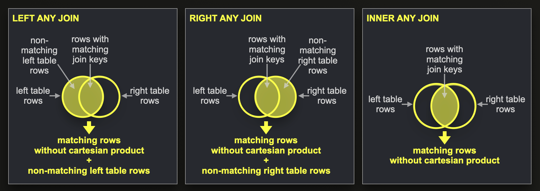
A LEFT ANY JOIN is the combination of the LEFT OUTER JOIN + the LEFT SEMI JOIN, meaning that ClickHouse returns column values for each row from the left table, either combined with the column values of a matching row from the right table or combined with default column values for the right table, in case no match exists. If a row from the left table has more than one match in the right table, ClickHouse only returns the combined column values from the first found match (the cartesian product is disabled).
Similarly, the RIGHT ANY JOIN is the combination of the RIGHT OUTER JOIN + the RIGHT SEMI JOIN.
And the INNER ANY JOIN is the INNER JOIN with a disabled cartesian product.
We demonstrate the LEFT ANY JOIN with an abstract example using two temporary tables (left_table and right_table) constructed with the values table function:
WITH left_table AS (SELECT * FROM VALUES('c UInt32', 1, 2, 3)), right_table AS (SELECT * FROM VALUES('c UInt32', 2, 2, 3, 3, 4)) SELECT l.c AS l_c, r.c AS r_c FROM left_table AS l LEFT ANY JOIN right_table AS r ON l.c = r.c; ┌─l_c─┬─r_c─┐ │ 1 │ 0 │ │ 2 │ 2 │ │ 3 │ 3 │ └─────┴─────┘ 3 rows in set. Elapsed: 0.002 sec.✎
This is the same query using a RIGHT ANY JOIN:
WITH left_table AS (SELECT * FROM VALUES('c UInt32', 1, 2, 3)), right_table AS (SELECT * FROM VALUES('c UInt32', 2, 2, 3, 3, 4)) SELECT l.c AS l_c, r.c AS r_c FROM left_table AS l RIGHT ANY JOIN right_table AS r ON l.c = r.c; ┌─l_c─┬─r_c─┐ │ 2 │ 2 │ │ 2 │ 2 │ │ 3 │ 3 │ │ 3 │ 3 │ │ 0 │ 4 │ └─────┴─────┘ 5 rows in set. Elapsed: 0.002 sec.✎
This is the query with an INNER ANY JOIN:
WITH left_table AS (SELECT * FROM VALUES('c UInt32', 1, 2, 3)), right_table AS (SELECT * FROM VALUES('c UInt32', 2, 2, 3, 3, 4)) SELECT l.c AS l_c, r.c AS r_c FROM left_table AS l INNER ANY JOIN right_table AS r ON l.c = r.c; ┌─l_c─┬─r_c─┐ │ 2 │ 2 │ │ 3 │ 3 │ └─────┴─────┘ 2 rows in set. Elapsed: 0.002 sec.✎
ASOF JOIN #

The ASOF JOIN, implemented for ClickHouse in 2019 by Martijn Bakker and Artem Zuikov, provides non-exact matching capabilities. If a row from the left table doesn’t have an exact match in the right table, then the closest matching row from the right table is used as a match instead.
This is particularly useful for time-series analytics and can drastically reduce query complexity.
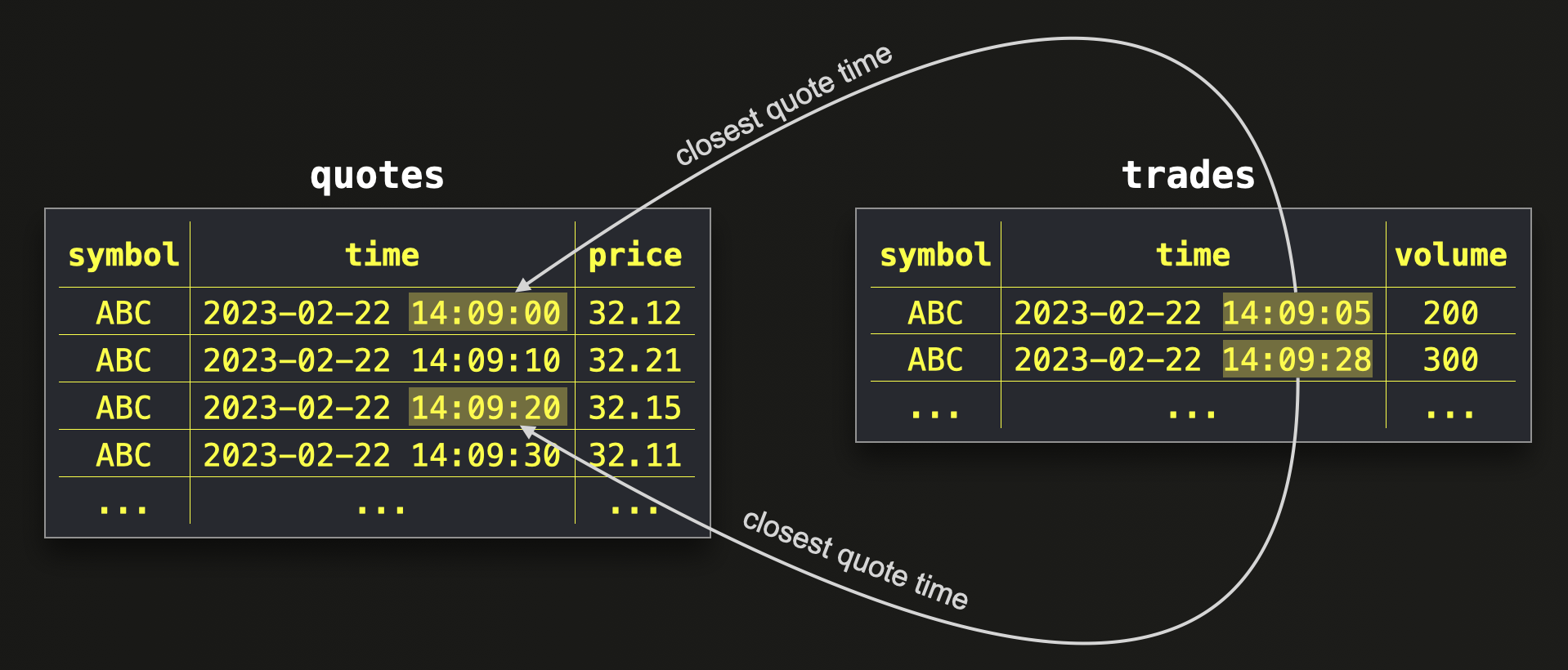
We will do time-series analytics of stock market data as an example. A quotes table contains stock symbol quotes based on specific times of the day. The price is updated every 10 seconds in our example data. A trades table lists symbol trades - a specific volume of a symbol got bought at a specific time:

In order to calculate the concrete cost of each trade, we need to match the trades with their closest quote time.
This is easy and compact with the ASOF JOIN, where we use the ON clause for specifying an exact match condition and the AND clause for specifying the closest match condition - for a specific symbol (exact match) we are looking for the row with the ‘closest’ time from the quotes table at exactly or before the time (non-exact match) of a trade of that symbol:
SELECT
    t.symbol,
    t.volume,
    t.time AS trade_time,
    q.time AS closest_quote_time,
    q.price AS quote_price,
    t.volume * q.price AS final_price
FROM trades t
ASOF LEFT JOIN quotes q ON t.symbol = q.symbol AND t.time >= q.time
FORMAT Vertical;

Row 1:
──────
symbol:             ABC
volume:             200
trade_time:         2023-02-22 14:09:05
closest_quote_time: 2023-02-22 14:09:00
quote_price:        32.11
final_price:        6422

Row 2:
──────
symbol:             ABC
volume:             300
trade_time:         2023-02-22 14:09:28
closest_quote_time: 2023-02-22 14:09:20
quote_price:        32.15
final_price:        9645

2 rows in set. Elapsed: 0.003 sec.
Note that the ON clause of the ASOF JOIN is required and specifies an exact match condition next to the non-exact match condition of the AND clause.
ClickHouse currently doesn't support (yet) joins without any part of the join keys performing strict matching.
Summary #
This blog post showed how ClickHouse supports all standard SQL JOIN types, plus specialized joins to power analytical queries. We described and demonstrated all supported JOIN types.
In the next parts of this series, we will explore how ClickHouse adapts classical join algorithms to its query pipeline to execute the join types described in this post as fast as possible.
Stay tuned!
Get started with ClickHouse Cloud today and receive $300 in credits. At the end of your 30-day trial, continue with a pay-as-you-go plan, or contact us to learn more about our volume-based discounts. Visit our pricing page for details.


