What's new in ClickStack. August '25.

We're now running ClickStack free in-person and online training. Some key dates for users looking to learn about the open source observability stack powered by ClickHouse:

Online Training – Wednesday, Aug 27 | 2–4 PM CEST
Training – Menlo Park, Wednesday, Aug 27
Training – San Francisco, Thursday, Aug 28

Welcome to the August edition of What’s New in ClickStack - the open-source observability stack for ClickHouse.

Each month, we share the latest updates across the stack, building on new ClickHouse features and HyperDX UI improvements that unlock fresh workflows, smarter visualizations, and a smoother user experience. This month’s release adds Cloud-hosted HyperDX, smarter search, dynamic visualizations, new SQL tricks, and cutting-edge inverted index support in ClickHouse - making ClickHouse observability faster, cleaner, and more powerful than ever.

New contributors #

Building an open-source observability stack requires a community. A big thank you to this month's new contributors! Every contribution, big or small, helps make ClickStack better for everyone.

Candido Sales Gomes, Toan Ho, Tomas Hulata, Anirudh, chenlujjj, João Spranger

ClickStack in ClickHouse Cloud #

The biggest news this month is that the HyperDX component of ClickStack is now available in ClickHouse Cloud (private preview).

This means simpler adoption for Cloud users - one less component to host yourself, and the UI now plugs directly into ClickHouse Cloud’s passwordless authentication. It also lays the groundwork for upcoming RBAC support and integrated alerting.

More importantly, it brings us closer to the ClickStack vision: the convergence of observability, real-time analytics, and data warehousing in a single, unified platform. In this vision, we see Logs, traces, and metrics being correlated directly with your business and application data in ClickHouse. With SQL as the language of choice, you can do things like quantify the financial impact of 400s and failed transactions - all in a simple SQL query.

That leaves just one piece of the stack you still need to host yourself: the OTel collector for ingestion. Stay tuned - we’re actively working on bringing this to the Cloud too.

For more details on the announcement and our vision for making observability just another data problem, check out our blog post: “Announcing ClickStack in ClickHouse Cloud: The first step to a future of unified observability and data analytics”.

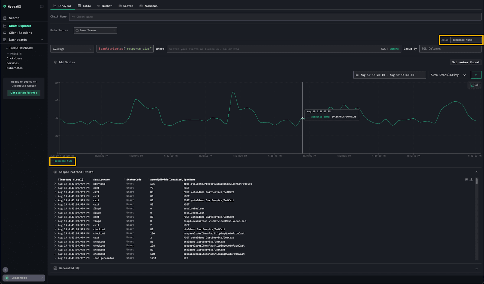
Custom chart alias’ #

Sometimes it’s the small features that make the biggest difference. HyperDX now lets you set custom aliases for chart axes - a simple but powerful addition, especially when working with complex expressions. The result? Cleaner charts with human-readable labels that make dashboards easier to understand at a glance.

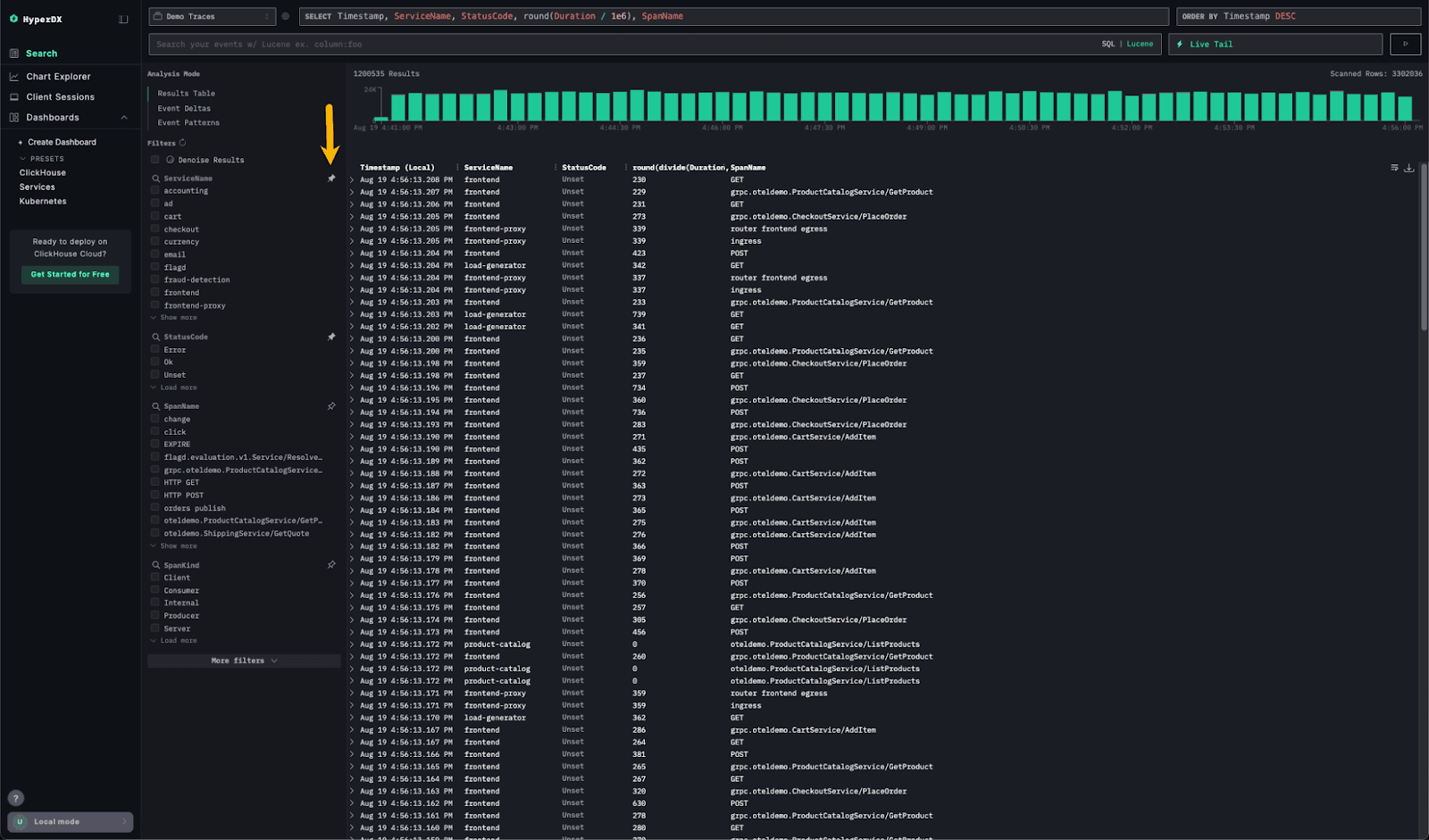
Pinned fields #

As ClickStack adoption grows, so does the feedback - and one theme we’ve heard loud and clear is around exploring and filtering data.

When searching logs or traces, users often apply filters while also tweaking search expressions. Root-cause analysis usually means keeping a close eye on a handful of key fields and watching how their values change as filters are applied.

The new Pinned Fields feature makes this much easier: fields of interest can now be pinned to the top of the left panel, reducing scrolling and keeping critical context always in view. A small change, but a big boost to workflow efficiency.

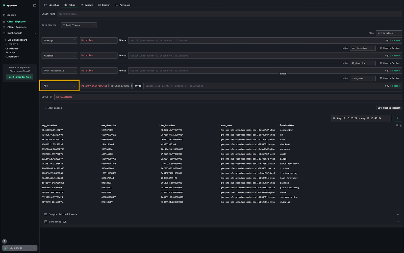
Support for Any aggregation #

Users familiar with ClickHouse SQL will appreciate the addition of the any aggregate function to HyperDX. This function is handy when you need to return the value of a column in an aggregation where a metric isn’t appropriate and any value will do.

It’s typically used alongside other aggregate functions, like min or max, to return a string label or non-numeric column.

For example, consider the following SQL query, which calculates the average, 90th percentile, maximum, and minimum performance for each service running in a Kubernetes cluster:

1SELECT
2    ServiceName,
3    avg(Duration) AS avg_duration,
4    max(Duration) AS max_duration,
5    quantiles(0.9)(Duration) AS `90_duration`
6FROM otel_v2.otel_traces
7GROUP BY ServiceName
8LIMIT 10

Suppose we also want to return the Kubernetes node name for each service in the aggregated results. In many cases, this is acceptable - either because there’s only one possible value (e.g. grouping by a unique key) or because any value provides enough context. We can modify the query as follows:

1SELECT
2    ServiceName,
3    any(ResourceAttributes['k8s.node.name']) AS node_name,
4    avg(Duration) AS avg_duration,
5    max(Duration) AS max_duration,
6    quantiles(0.9)(Duration) AS `90_duration`
7FROM otel_v2.otel_traces
8GROUP BY ServiceName
9LIMIT 10

Effectively, the any function avoids the need to add the column to the GROUP BY - in turn avoiding the increase in the cardinality of the aggregation and associated memory overhead.

Now, ClickStack users will rarely write raw SQL like the example above when exploring data. However, the any aggregate makes it possible to build richer tables more efficiently - without having to aggregate by every single field just to return a value.

For example, we can create a table using the any function that reproduces the results of the above query:

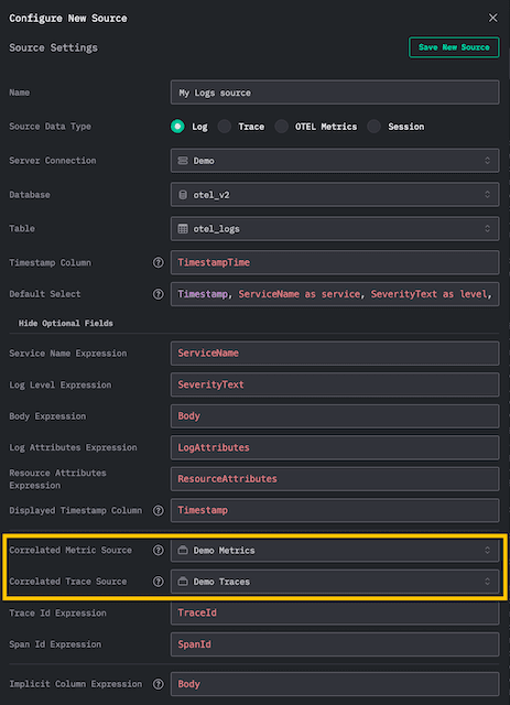
Auto-correlated sources #

Sources in HyperDX represent a database and table from a specific ClickHouse instance - the foundation on which all searches and charts are built.

When you create a source, it can be connected with another source of a different type. This tells HyperDX that the two datasets belong to the same observability context and can be correlated visually in the UI.

This concept is key to delivering the “single pane of glass” experience: unifying logs, metrics, and traces so they can be explored together. For example, this enables you to view logs in the context of a trace and vice versa.

Importantly, these connections had to be declared in both directions.

When using the default OTEL schemas, sources for Logs, Traces, and Metrics are created automatically, and these bi-directional connections are set up for you.

However, many users deviate from the defaults - often to work with their own wide events. In these cases, creating a data source is a manual exercise, and correlating two sources has traditionally required a multi-step process. More specifically:

1. Create the first data source (e.g. Logs)
2. Create the second data source (e.g. Traces) and specify that it’s correlated with the Logs source
3. Go back and modify the Logs source to declare the correlation with Traces

In the latest version of ClickStack, this workflow is much simpler thanks to auto-correlated sources. Step 3 is now handled automatically - when a user declares a connection from one source to another in step (2), the reverse connection is created for you.

For users managing a large number of sources, often across multiple data versions, this change greatly simplifies setup and reduces the chance of errors, ensuring more consistent data across the application.

Improved query efficiency for time-based primary keys #

In large-scale ClickStack deployments, it’s common to tune the primary key by making toStartOf[Minute|Hour|etc)(Timestamp) the first column, followed by fields like ServiceName and the high-granularity timestamp. This design aligns with ClickHouse best practices and makes time-based filtering far more efficient.

Previously, the HyperDX UI didn’t fully exploit this when returning the "latest" results. Queries ordered by the raw Timestamp alone did not align with the sorting key, forcing ClickHouse to scan more granules than necessary. Effectively, this prevented ClickHouse from using optimize_read_in_order, where the server leverages the table index to read rows in primary key order. With this optimization, queries on large datasets with a small LIMIT (like in HyperDX) can be executed much faster.

The latest release fixes this with added intelligence in the search layer of HyperDX. When a toStartOfMinute (or equivalent) expression is detected in the primary key, HyperDX now automatically orders results beginning with this column (e.g. ORDER BY toStartOfMinute(Timestamp) DESC, Timestamp DESC).

This allows ClickHouse to use the sorting key directly and read data in order, avoiding unnecessary scans. Queries that once required reading millions of rows can now return the same results after touching only a fraction of the data.

For example, consider the following table of 100 million random integers populated with the INSERT INTO SELECT:

1CREATE TABLE random_integers
2(
3    `value` DateTime,
4    `name` String
5)
6ENGINE = MergeTree
7ORDER BY (toStartOfMinute(value), name, value)
8
9INSERT INTO random_integers SELECT
10    value,
11    'asdf' AS name
12FROM generateRandom('value Int32')
13LIMIT 100000000

If we select the top 10 rows and order by value, note how all 100 million rows are read:

1SELECT * from random.random_integers
2  ORDER BY value DESC
3  LIMIT 10

Conversely, if we order by (toStartOfMinute(value), name, value) we read a fraction of the number of rows - improving the response time:

1SELECT *
2FROM random.random_integers
3ORDER BY (toStartOfMinute(value), value) DESC
4LIMIT 10

Chart display switcher #

Picking the right visualization isn’t always straightforward - the “best” chart often depends on the data you’re looking at, and that can change once filters are applied. A chart that works perfectly for the full dataset might fall short when zooming into a subset.

Most tools lock you into a chart type when you create it, leaving you stuck if it no longer fits the view.

With the latest release, ClickStack adds dynamic chart type switching. You can now toggle between bar and line charts right on the dashboard - even after a visualization has been added. No need to rebuild the chart, just switch to the view that best fits your data.

We’re already exploring other chart pairings that naturally complement each other - and plan to expand this feature to more visualization types wherever workflows overlap.

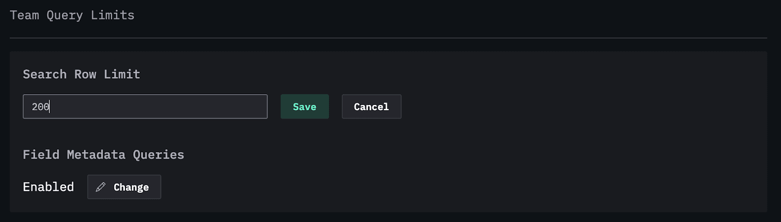
Search limit support #

By default, HyperDX returns 200 rows per search - a sensible balance between server load and giving users enough context. But on very large datasets, even this can be heavy. Conversely, in other cases, users may have sufficient resources and simply want to see more results at once.

With the latest ClickStack release, this limit is now configurable. The default is still 200, but you can dial it up or down to match your performance needs and preferred level of visibility.

Inverted indices support #

So far, we’ve focused on HyperDX improvements. But ClickStack also continues to benefit from developments in ClickHouse itself - the engine behind the performance and scalability we all love.

One particularly relevant update for observability workloads is the announcement that the inverted indices skip index has undergone significant improvements. This feature has existed experimentally for some time, but after major rework, it’s now compatible with ClickHouse Cloud and available in private preview.

Inverted indices promise faster full-text search, a common need when querying log bodies. But whether they’re worth the cost has long been debated:

• Do the storage and generation overheads justify the performance gains?

• Are the data structures efficient enough for object storage?

Until now, ClickHouse has supported full-text search through Bloom filters and linear scan techniques. Bloom filters offered lightweight skipping for keyword searches, but came with tuning complexity and the risk of false positives, as well as a lack of support for multi-token search. Linear scans, by contrast, directly searched text columns. These worked reliably but required scanning large amounts of data, making them slower at PB scale.

Recent work has reimagined full-text search in ClickHouse with a new index that combines data structures such as finite state transducers (FSTs) for efficient token dictionaries and roaring bitsets for highly compressed posting lists and set operations (e.g. for disjunctions and conjunctions). This pairing allows for faster, more accurate text lookups while drastically reducing storage overhead. The result is an inverted index that promises significant improvements in query performance, scalability, and efficiency, all while being exposed through a simpler and more intuitive syntax that avoids the manual tuning Bloom filters once required.

Until the feature matures, the default OTel schema remains unchanged - we’re testing, benchmarking, and gathering feedback to answer key questions:

• Is the extra storage and I/O worth it for observability?

• Do insert and merge times increase enough to require more compute, and is that justified by faster queries?

• Should inverted indices be applied only to recent data, or does object storage make the additional storage overhead irrelevant?

Interesting, the implementation actually still exploits Bloom filters for a lightweight check as to whether a term exists, allowing full evaluation of the index to be skipped if the filter reports the term as not being present in a granule - relying on the fact that false negatives are impossible.

We highly recommend the blog from our engineering team for more details on the implementation details and challenges of adding inverted indices to a column store.

Early signs are promising, but the principle remains: skip indices are optional and applied at the column level. Unlike systems where inverted indices are core to the design, ClickStack users will always have a choice - armed with the knowledge to enable them where they make sense.

Stay tuned - we’ll be sharing more benchmarks and insights over the coming months as we get closer to answering the question: when does observability really need inverted indices?

In the meantime, please feel free to enable inverted indices on your Body column and let us know how it performs!