Inside ClickHouse full-text search: fast, native, and columnar

TL;DR

We’ve completely rebuilt full-text search in ClickHouse, faster, leaner, and fully native to the columnar database design.

This is a deep technical dive by the engineers who built it, covering the new design from inverted indexes to query-execution tricks that skip reading the text column entirely. If you care about high-performance search without leaving your database, or love seeing database internals stripped bare, this one’s for you.

From legacy to lightning-fast: the journey of ClickHouse full-text search #

Full-text search (FTS) isn’t new to ClickHouse, but until now it ran on an older implementation with limits in performance and flexibility. We’ve gone back to the drawing board and re-engineered it from scratch, making search faster, more space-efficient, and deeply integrated with ClickHouse’s columnar design.

You can register for the private preview of the rebuilt full-text search by following this link

This is your under-the-hood tour, showing the core data structures — inverted indexes, finite state transducers, posting lists — and how the query pipeline was redesigned to cut I/O and speed up searches.

If you’ve ever needed to:

• run search-like analytics directly inside ClickHouse,

• avoid maintaining a separate search engine, or

• understand how modern text indexing works in a column store,

…you’ll get both the why and the how, backed by real examples and measurable performance gains.

Let’s start by looking at how the new index stores and organizes text, the foundation for everything that follows.

What makes full-text search fast? #

Imagine you’re storing product reviews, log messages, or user comments in ClickHouse. Each row contains a natural language document, i.e. a text written by human or a machine that follows a natural language grammar (no random IDs, no hash values).

Because ClickHouse is a column-oriented database, we store these documents one after another in a column of type String. Each row holds a single document, which we can later search.

To make the content searchable, we split every document into a series of tokens, typically words. For example, the sentence:

All cats like mice

…would be tokenized as:

[All, cats, like, mice]

The default tokenizer splits strings by spaces or punctuation. More advanced tokenizers can split log messages into their components, for example, timestamp, severity, and message fields, or even extract n-grams for fuzzy search.

A full-text search then retrieves documents that contain a specific token. For example, to find the rows which mention cat, we might run:

SELECT [...] FROM [...] WHERE documents LIKE '% cat %'

(Notice the spaces — without them, we might accidentally match “educate” or “multiplication.”)

Full-text search can be implemented in two ways:

• Full scans – scan every row (slow)

• Inverted indexes – map each token to its containing rows (fast)

Inverted indexes make it possible to search massive datasets in milliseconds, and that’s exactly what ClickHouse now supports natively, with scale and performance in mind.

Before we dive into the details of how it works, let’s unpack the name “inverted index”, a simple idea that flips the usual document → terms mapping on its head, but can seem counter-intuitive if you’ve never worked with search engines before.

Why is it called an inverted index? #

When you read multiple documents from beginning to end, you can remember for each document the (unique) terms it contains. This document → terms mapping is sometimes called forward index.

An inverted index search flips that around: It stores a term → documents mapping. Given a term, it allows you to find all documents that contain it.

It’s like the back of a book: instead of reading pages to find a word, you look up the word to see which pages it’s on. That reverse lookup is what makes search engines fast, and it’s built into ClickHouse.

Now that we know what an inverted index is, it’s worth looking at where ClickHouse started. ClickHouse has always had ways to speed up text lookups, but these were approximations. To see why a true inverted index was needed, let’s trace the evolution from our earlier Bloom-filter-based approach to the new design.

From bloom filters to real indexes #

Before introducing native text indexes, ClickHouse already supported full-text search using the "bloom_filter" "tokenbf_v1" and "ngrambf_v1" indexes. These are based on Bloom filters, a probabilistic data structure for checking whether the indexed documents contain a value.

Compared to inverted indexes, Bloom filters come with a few key limitations:

• Hard to tune: Using a Bloom filter requires manual tuning of the byte size, the number of hash functions, and an understanding how they affect the false positive rate. This often requires deep expertise.

• False positives: Bloom filters may answer that a value might exist even when it doesn’t. This means that additional rows have to be scanned, reducing efficiency of the search.

• Limited functionality: Bloom filter indexes only support a small subset of expressions in the WHERE clause, while inverted indexes are, in principle, more versatile.

Inverted indexes solve all three of these issues, and that’s why they now power full-text search in ClickHouse.

How the new text index works #

To understand how the new engine achieves its speed and precision, we first need to look at how the index is organized on disk and how queries interact with its building blocks.

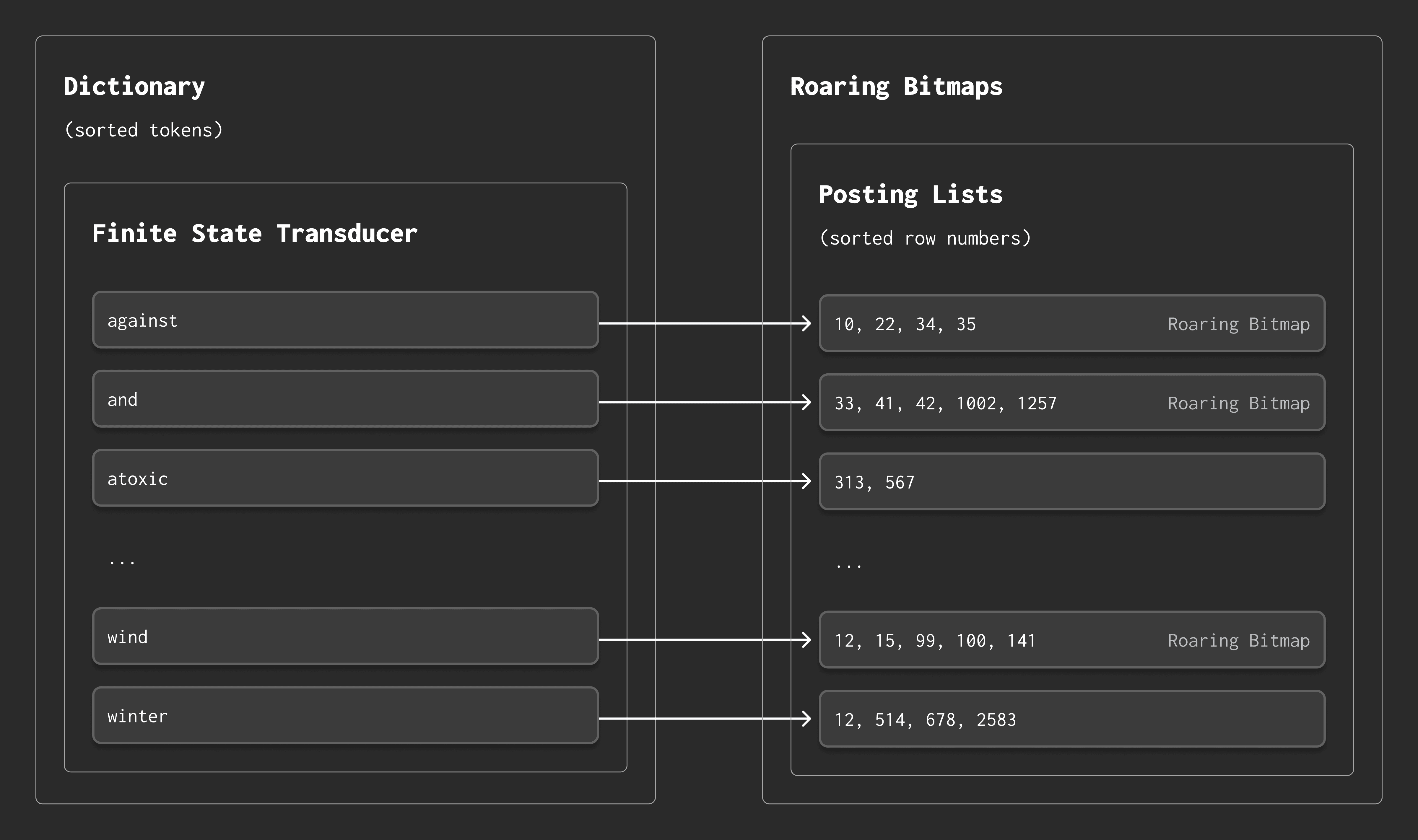
Index structure: dictionaries + posting lists #

ClickHouse’s full-text search is powered by a native inverted index, also known as a text index. Conceptually, this index consists of two key components:

1. A dictionary, storing all unique tokens across all documents.

2. Posting lists, which record the row numbers of documents that contain each token.

Here’s how it works:

• When you search for a token, ClickHouse looks it up in the dictionary.

• If it is found, the dictionary returns the location of the corresponding posting list.

• The posting list is simply a list of row numbers — i.e., the documents — that contain that token.

  Example:

• The token wind might appear in documents 12, 15, 99, 100, and 141.

• The token winter might appear in documents 12, 514, 678, and 2583.

This index design makes token lookups fast and efficient — even at massive scale.

Below is a simplified diagram of this structure:

Under the hood, ClickHouse stores and compresses both the dictionary and the posting lists using advanced data structures, which we’ll explore next.

FSTs: Space-efficient dictionaries #

To find a token quickly, we need an efficient dictionary structure.

The most basic approach for this is a sorted list of (token → posting list) pairs. This lets us do a fast binary search to find a token. Assuming that the documents are written in natural language, this opens up another useful optimization opportunity: prefix sharing.

For example, many tokens start with the same prefix:

• "wind", "winter"
• "click", "clickhouse"

A plain list of tokens doesn’t take advantage of this - but a Finite State Transducer (FST) does.

What is an FST? #

An FST is a compact automaton—essentially a graph of characters—that encodes the dictionary in a highly compressed manner. It was originally designed to translate strings from one language to another, but it is also a great fit for text indexing. Systems like Lucene and ClickHouse use FSTs to represent sorted dictionaries.

Instead of storing each token as a string, an FST:

• Represents shared prefixes and suffixes only once

• Encodes each token as a path through a graph

• Emits an output (e.g. the address of a posting list) when a path reaches a final “accepting” state.

This makes the dictionary extremely compact, especially when tokens share common parts.

Mapping tokens to posting lists #

The FST doesn’t store the posting lists themselves — just how to find them. For that, we associate each token with a posting list offset: the byte position where it begins in a separate file.

To retrieve the offset for a token, we walk the FST from the start state to an accepting state. Each transition may emit an integer, and we sum them all to get the final offset. This sounds a bit magical, but it’s how the standard FST construction algorithm works (ref).

Example #

Suppose we have three tokens:

ClickBench, ClickHouse, JSONBench

We’ll build the FST for the following small dictionary and see how the FST looks visually.

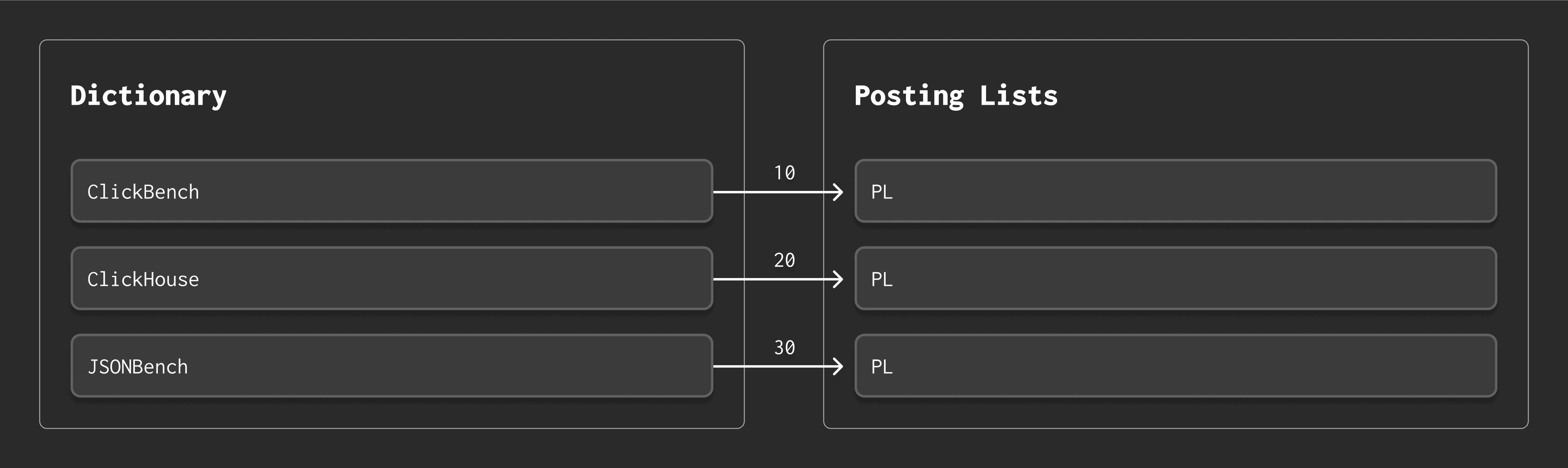
The FST encodes the tokens as transitions between characters. Shared prefixes like "Click" reuse the same path. At the end of each token, the FST emits its corresponding offset (10, 20, 30):

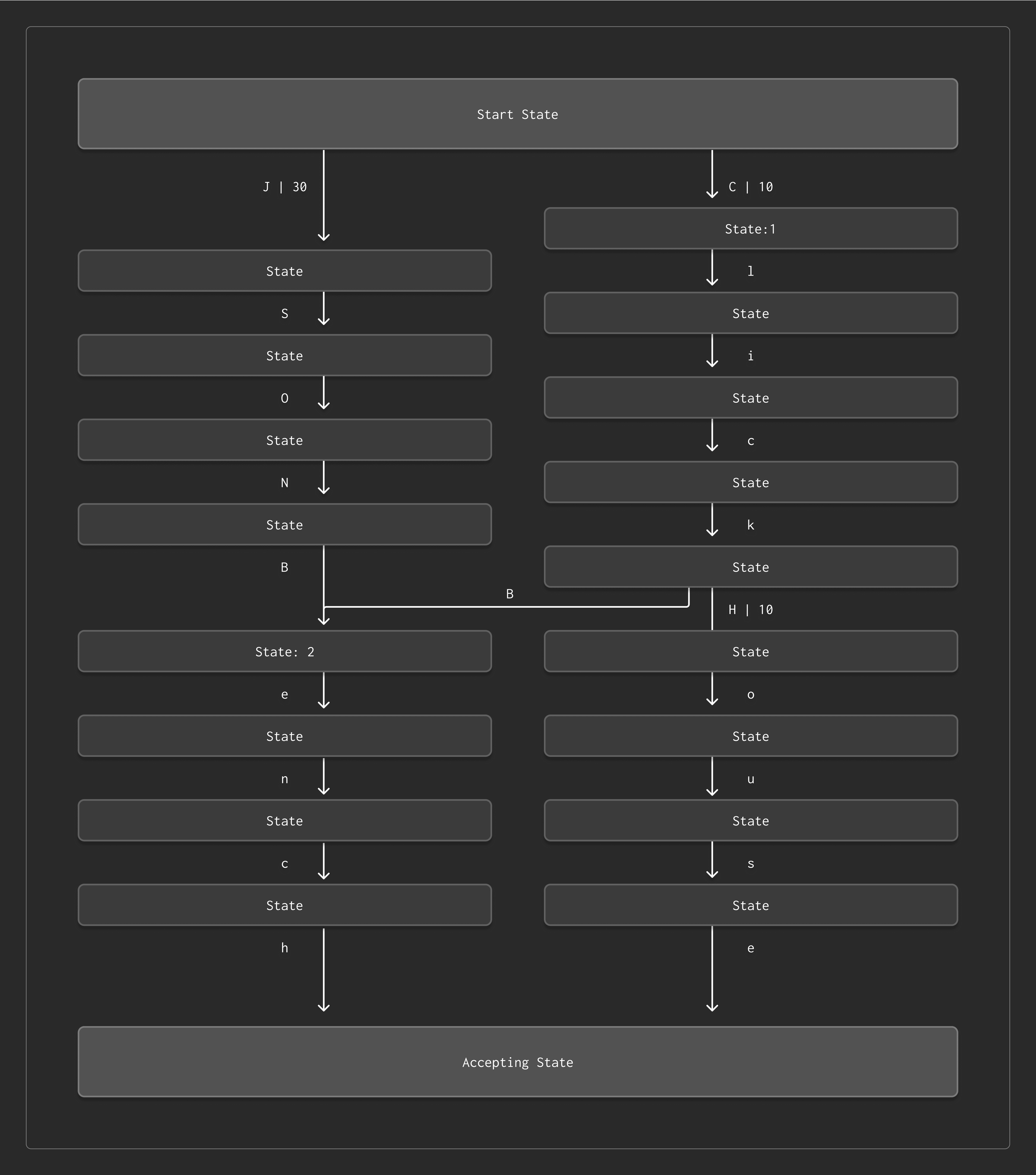
So the FST serves two roles:

• It lets us quickly check whether a token exists.

• It lets us compute the byte offset for that token’s posting list.

Together, this allows ClickHouse to store large token dictionaries in a compact and searchable manner.

Roaring bitmaps: fast set operations #

Each posting list stores the row numbers of documents that contain a given token.

We want to store these row numbers in a way that’s:

• Compact – to save space.

• Efficient – so we can quickly compute intersections and unions between posting lists.

Posting list intersections and unions matter when queries involve multiple tokens and combine them with logical operators, e.g.:

LIKE '% cat %' AND LIKE '% dog %'

Why Compression Matters #

The traditional approach for compressing posting lists is to combine:

• Delta encoding – to calculate the differences between neighboring values.

• Golomb-Rice encoding – to compress the deltas efficiently.

This scheme offers excellent compression for typical natural language documents (a few frequent tokens and many rare ones). However, it processes data bit by bit, which isn’t ideal for modern CPUs that benefit from pipelining and SIMD instructions.

Enter roaring bitmaps #

To keep things fast, ClickHouse uses Roaring bitmaps, a modern, high-performance format for storing large sets of integers.

The idea is simple:

• Think of a posting list as a bitmap, e.g., [3, 5, 8] → 000101001

• Divide the bitmap into chunks of 65,536 values (2¹⁶).

• Store each chunk in a specialized container, based on its content:

  • Array – for sparse data (few values)

  • Bitmap – for dense data

  • Run-length encoding – for long consecutive sequences

This design keeps storage compact and enables extremely fast set operations — including all combinations of AND, OR, and NOT between posting lists. Roaring bitmaps also use specialized SIMD-accelerated code paths for maximum speed.

Visual breakdown #

Roaring bitmaps split each 32-bit row number into two 16-bit parts:

• The upper 16 bits select the container.

• The lower 16 bits are stored inside the container.

For example:

• Row number: 124586

• Binary: 00000000 00000001 11100110 11101010

• Upper 16 bits: 00000000 00000001 → selects container

• Lower 16 bits: 11100110 11101010 → value stored in container

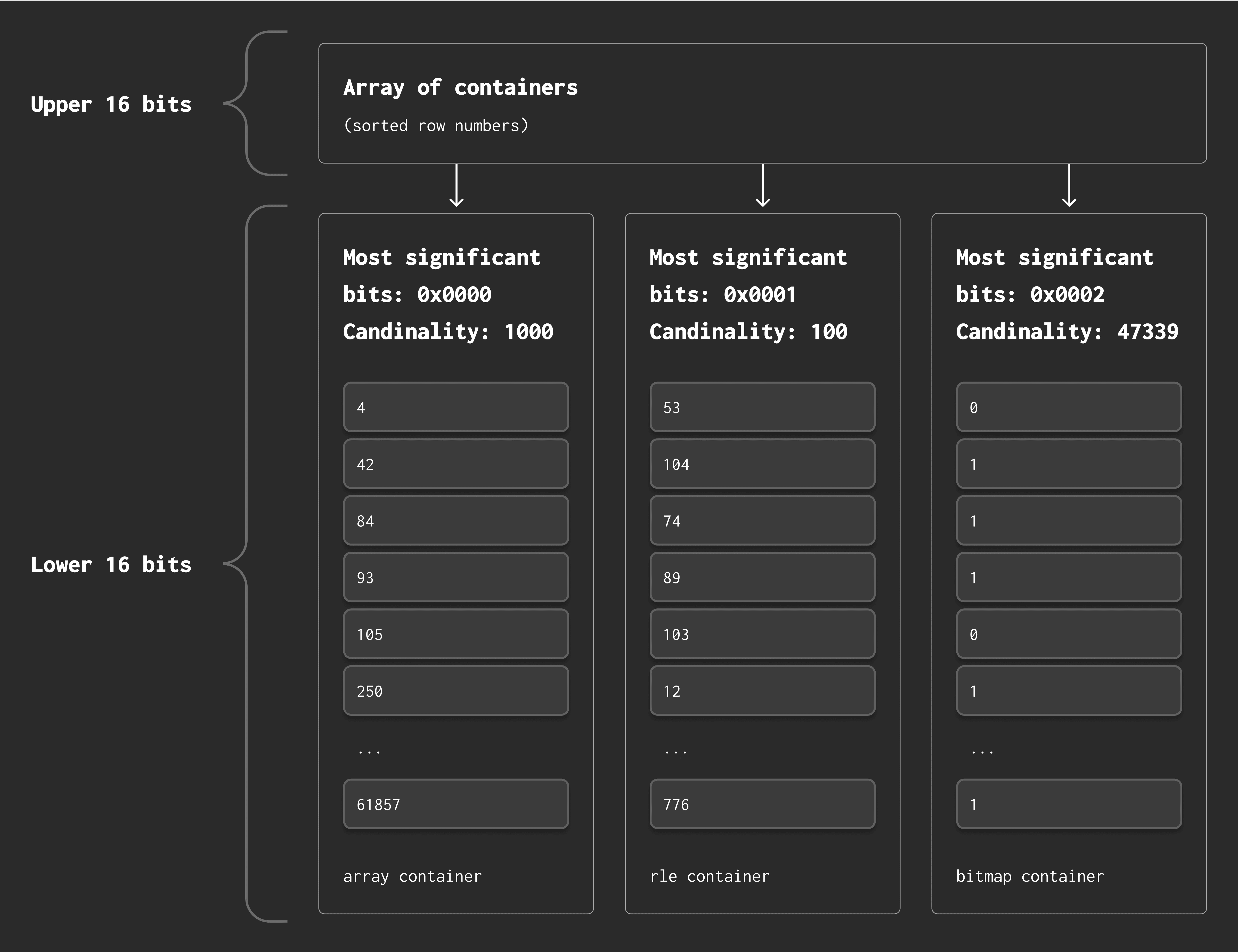
Each container holds values for a specific range and is stored using the most space-efficient format. This makes it possible to scan, merge, and filter billions of row numbers with blazing speed.

We now have the two core building blocks of ClickHouse’s text index:

• FSTs for compact, prefix-sharing token dictionaries

• Roaring bitmaps for fast, compressed posting lists

We’ve now covered the two core structures — the dictionary and the posting lists — and how they’re stored efficiently. Let’s put these pieces together and see how the index is organized on disk.

Storage layout: segments, granules, and files #

Let’s put all the pieces together.

An inverted index consists of five files on disk:

1. An ID file — stores the segment ID and version. (see below what "segment" means)

2. A metadata file — tracks all the segments.

3. A bloom filter file — stores bloom filters to avoid loading dictionary and posting list files.

4. A dictionary file — stores all segment dictionaries as FSTs.

5. A posting list file — stores all posting lists as compressed sequences of integers.

See the next diagram for an overview of how these pieces are laid out on disk.

How the Data is Organized #

The index is built per part and recreated during merges. Internally, it’s split into segments, each of which contains:

• A dictionary (as an FST)

• Posting lists (as roaring bitmaps), one per token

The metadata file keeps track of:

• The segment ID

• The starting row ID

• Offsets into the Bloom filter file, dictionary file, and posting list file

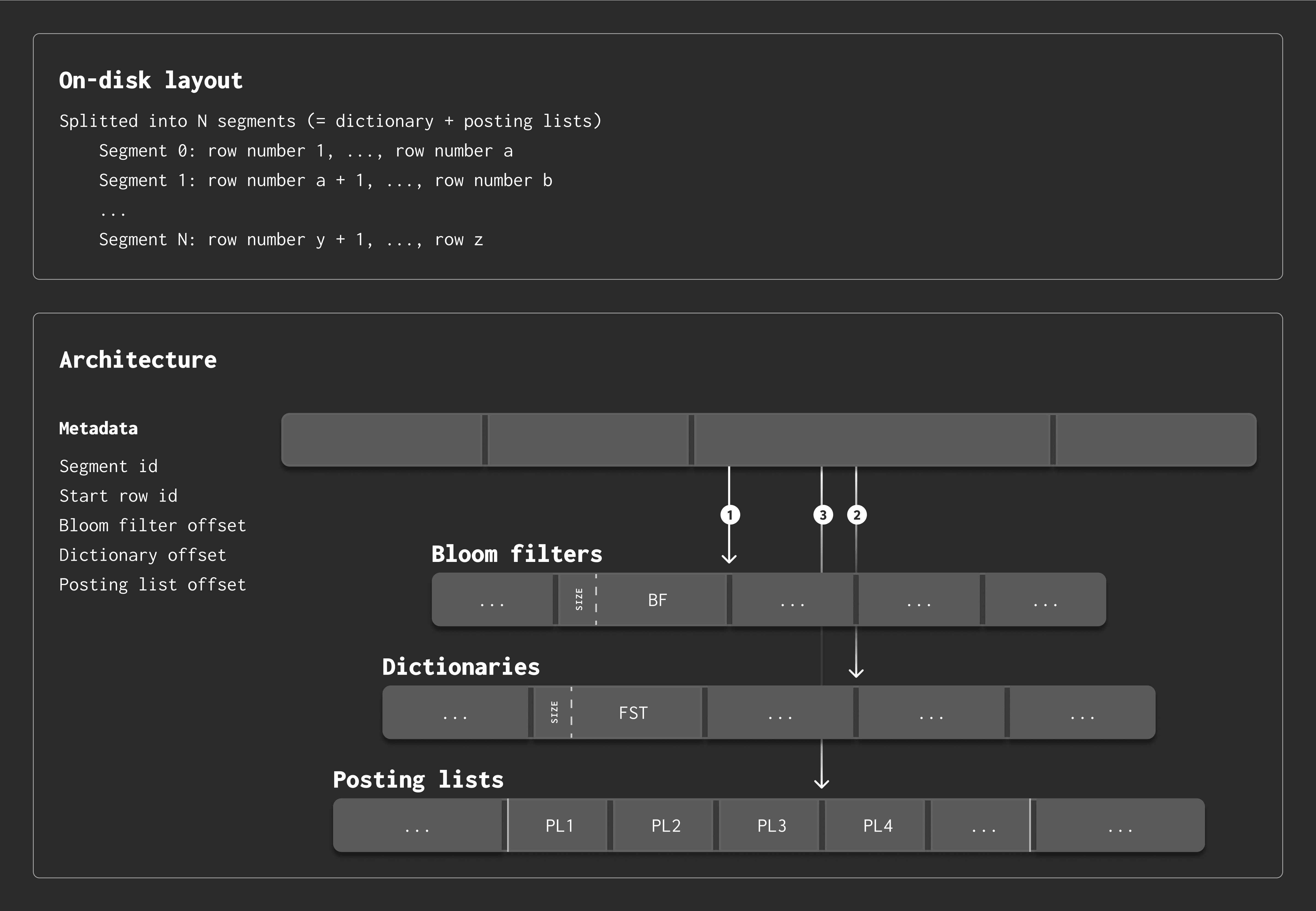
In the diagram above, arrows marked ①, ②, and ③ represent the order in which files are loaded during lookups.

We shape the file sizes to match their content:

• Bloom filters are the smallest,

• Dictionaries are mid-sized,

• Posting lists are the largest.

What’s a Segment? And What’s an Index Granule? #

To understand segments, we need to introduce index granules.

• An index granule is the unit of indexing in ClickHouse (typically 8192 rows).

• A segment is a substructure within the granule, created to make indexing more memory-efficient.

Segments are split by dictionary size, not by row count. This makes sure that each segment holds FST dictionaries of roughly the same size. This approach avoids out-of-memory errors during index creation on large datasets.

Each segment is self-contained and holds:

• A row ID range

• An FST dictionary

• A set of posting lists

Smaller segments reduce memory pressure, but may lead to higher storage usage due to redundant storage of tokens in multiple segment FST dictionaries. Segmenting is off by default but can be enabled for advanced workloads.

What happens during an index lookup? #

Here’s how ClickHouse finds rows for a search token:

1. Traverse all dictionaries:

The token is searched in every segment’s FST. When the FST reaches its accepting state, we know the token exists in that segment.

2. Sum up FST output values:

These values give us the offset into the posting list file.

3. Load the posting list:

   • If it’s a cold run, the posting list is read from disk.

   • If it’s a hot run, it’s already cached in memory.

   Note: The row IDs stored in posting lists are relative to the segment’s starting row. They’re extrapolated to full granule row numbers during lookup. (More on that in direct index usage optimization below.)

With the fundamentals in place, let’s look at the major improvements we’ve made to the text index in this release, covering everything from API design to memory footprint and smarter granularity.

Recent improvements #

Over the past three months, we’ve made significant improvements to full-text search in ClickHouse, from user-facing changes to deep storage optimizations. Here’s what’s new (and what’s coming):

1. A cleaner API #

We renamed the index from “inverted” to “text” and reworked the syntax to be more intuitive.

You can now pass parameters as key-value pairs directly in the INDEX clause. This makes the index both easier to use and more flexible.

CREATE TABLE tab
(
    [...],
    documents String,
    INDEX document_index(documents) TYPE text(tokenizer = 'default')
)
ENGINE = MergeTree
ORDER BY [...];

This creates a text index using the default tokenizer (which splits text by non-alphanumeric characters). You can also specify alternate tokenizers like 'ngram', 'split', and 'no_op', and provide additional settings like the n-gram size.

2. New split tokenizer #

We’ve added a new tokenizer type called split that is designed for semi-structured text such as logs or CSV-style data.

Unlike the default tokenizer, which tries to identify words based on general rules, the split tokenizer only breaks text at specific separators you define (by default: ,, ;, , \n, and \\).

This makes it ideal for:

• CSV-style input

• Log messages with consistent delimiters

• Any scenario where you want precise control over token boundaries

Example: CSV-style input #

Let’s compare the default tokenizer with the new split tokenizer for a CSV-style string

SET allow_experimental_full_text_index = 1;

CREATE TABLE tab_csv_default (
  id Int64,
  str String,
  INDEX idx_str(str) TYPE text(tokenizer = 'default'])
)
ENGINE = MergeTree()
ORDER BY id;

CREATE TABLE tab_csv_split (
  id Int64,
  str String,
  INDEX idx_str(str) TYPE text(tokenizer = 'split', separators = [',', ';', '$'])
)
ENGINE = MergeTree()
ORDER BY id;

Insert a multi-line CSV-style value:

INSERT INTO tab_csv_default (id, str) VALUES
(1,
'Click
House,ClickHouse,JSONBench'
);

INSERT INTO tab_csv_split SELECT * FROM tab_csv_default;

What changes with split #

The default tokenizer sees the above value as the tokens:

['Click', 'House', 'ClickHouse', 'JSONBench']

It ignores the newline between “Click” and “House”, so "Click\nHouse" is not treated as one token.

The split tokenizer, however, only splits where separators match exactly, so it keeps "Click\nHouse" together.

Searching #

Default tokenizer → no match for the multi-line token:

SELECT * FROM tab_csv_default WHERE searchAny(str, ['Click\nHouse'])

Ok.

0 rows in set. Elapsed: 0.001 sec.

Split tokenizer → correctly finds it:

SELECT * FROM tab_split WHERE searchAny(str, ['Click\nHouse'])


┌─id─┬─str────────────────────────┐
│  1 │ Click                     ↴│
│    │↳House,ClickBench,JSONBench │
└────┴────────────────────────────┘

1 row in set. Elapsed: 0.003 sec.

Key takeaway:

Use the split tokenizer when you need exact, separator-based tokenization and want to preserve multi-line or unusual token boundaries.

3. Smaller index footprint #

We made major improvements to reduce the memory and disk footprint of text indexes:

• PFOR compression for posting lists Fast intersection and union operations on posting lists are only performed on posting lists in memory. For posting lists stored on disk, we can sacrifice this requirement in favor of higher compression ratios. We therefore now use PFOR (Patched Frame of Reference) on top of Delta encoding. This change alone reduced their storage footprint by up to 30%.

• Zstd compression for FSTs FSTs are now Zstd-compressed when written to disk, lowering their average size by an additional 10%.

4. Cloud compatibility #

The text index is now fully compatible with ClickHouse Cloud, including support for the packed part format used in cloud storage.

5. Smarter granularity #

We increased the default index granularity from 1 to 64.

The index granularity determines how many rows are covered by each index granule:

Granularity docs →

• Smaller granularity: More precise filtering, but higher memory usage and I/O due to redundant storage of tokens in multiple FSTs.

• Larger granularity: Less overhead, better performance for most terms, but slightly less precision for very rare or clustered tokens.

Through extensive experiments, a setting of 64 delivered strong performance across both typical and edge-case workloads, making it the new default.

Beyond these core improvements, we’ve also added new capabilities to make lookups faster and lighter, starting with bloom filters as a pre-filtering layer.

6. Bloom filters as pre-filters #

Bloom filters are lightweight, probabilistic data structures that support efficient “one-way” set membership tests. They can quickly tell you:

• Definitely not in the set, or

• Possibly in the set (with a tunable false-positive rate)

Because they never return false negatives, bloom filters are useful for cheaply ruling things out before doing more expensive work.

In ClickHouse, we added bloom filters as pre-filters for the text index. This means we can check whether a token is definitely not in the dictionary before scanning the FST. That helps reduce disk I/O and CPU overhead. Since bloom filters are small, they can stay in memory at all times.

Text index vs bloom filter index: what’s the difference? #

There are two ways to use bloom filters in full-text search:

1. A bloom filter text index, where tokens are inserted directly into the bloom filter

2. A bloom filter on top of a text index segment, initialized from the segment dictionary

We mentioned the disadvantages of bloom-filter based indexes above - the most important downside is that these indexes require manual tuning.

The second way is fully automatic based on the indexed data and a configurable false positive rate (default: 0.1%) - no manual tuning is needed, meaning it easy to use and suitable for most scenarios.

In general, we recommend using text indexes over bloom filters unless you have specific accuracy needs.

While bloom filters speed up the decision of whether to check a dictionary, we’ve also improved how you query the index with new search functions.

7. New search functions: searchAny and searchAll #

Modern problems require modern solutions.

As ClickHouse added additional tokenizers and tokenizer-specific parameters, it turned out that the existing “hasToken” function is limited: it always uses the default tokenizer to tokenize the search term, not the tokenizer used to build the index. That can be unintuitive, and we’ve fixed it.

We’ve introduced two new functions for full-text search: searchAny and searchAll.

A simple example #

Let’s say we create a table like this:

SET allow_experimental_full_text_index = 1;

CREATE TABLE tab (
  id Int64,
  str String,
  INDEX idx_str(str) TYPE text(tokenizer = 'ngram', ngram_size = 5)
)
ENGINE = MergeTree()
ORDER BY id;

INSERT INTO tab (id, str) VALUES
  (1, 'Click House'),
  (2, 'ClickHouse');

Now, using the old hasToken function:

SELECT * FROM tab WHERE hasToken(str, 'Click');
┌─id─┬─str─────────┐
│  1 │ Click House │
└────┴─────────────┘

Why?

hasToken requires a non-alphanumeric separator before and after the token. Since “ClickHouse” has no separator, it’s not matched.

Try searchAny instead:

SELECT * FROM tab WHERE searchAny(str, ['Click']);

Returns both rows:

┌─id─┬─str─────────┐
│  1 │ Click House │
│  2 │ ClickHouse  │
└────┴─────────────┘

searchAll would do the same in this case.

Why are these better? #

No separator requirement

The new functions don’t require special characters around tokens. They use the tokenizer from the index itself.

Support for multiple tokens

Instead of writing:

SELECT * FROM tab WHERE hasToken(str, 'Click') AND hasToken(str, 'House');

SELECT * FROM tab WHERE hasToken(str, 'Click') OR hasToken(str, 'House');

You can now write:

SELECT * FROM tab WHERE searchAll(str, ['Click', 'House']);

SELECT * FROM tab WHERE searchAny(str, ['Click', 'House']);

Cleaner syntax and fewer surprises

These functions always use the tokenizer and settings defined in the index.

searchAny and searchAll only work with columns that have a full-text index. See searchAny docs and searchAll docs for more.

These new functions make searching more flexible and intuitive, but the biggest performance leap comes from a new optimization that skips reading the text column entirely.

Fast row-level search without text column reads #

ClickHouse's inverted index is at its core a skip index. As such, it is used at the beginning of a search to filter out non-matching granules. The "surviving" potentially matching granules are then loaded in a second step from disk and filtered row-by-row. In the case of the inverted index, this works well if the user searches a rare term. However, frequent terms cause many, potentially all, granules to survive and effectively a full scan in the second step.

What’s new? #

We’ve now eliminated that bottleneck.

The inverted index can now filter directly using the index, down to the row level.

This means we no longer need to read the text column at all.

It builds on the existing granule-level filtering logic and introduces a new match engine that’s completely transparent to users.

Example #

Consider the query:

SELECT col1, col2 FROM table WHERE searchAny(col3, ['hello'])

Before: Read the text column to match rows #

• The engine had to read col3 (the indexed text column) to filter the surviving granules row by row.

• Even with index filtering at the granule level, this still involved reading and scanning many rows.

• That’s slow, especially since text columns are large, and row-level filters were missing.

After: Use the index only — up to 10x faster #

• Now we read only the index.

• The engine uses the index to extract matching row IDs, skipping col3 entirely.

• Only the requested columns (col1, col2) are read.

• This cuts out 90%+ of query time for frequent terms.

To visualize the change, here’s a side-by-side sketch of the old vs new execution path.

This diagram shows how queries were executed before the optimization.

To evaluate hasToken(col3, 'hello'), ClickHouse had to:

• Read granules from the col3 text column to find matching rows.

• Read col1 and col2 as well to return the full result.

Although the index was already used to skip granules, it couldn’t fully filter at the row level.

As a result, we still had to scan and parse text row by row to apply match logic — even though the index already had that information.

This was inefficient, especially for large text columns, because:

• Text columns tend to be large and costly to read.

• The index already stored the necessary match data in a much smaller, more efficient format.

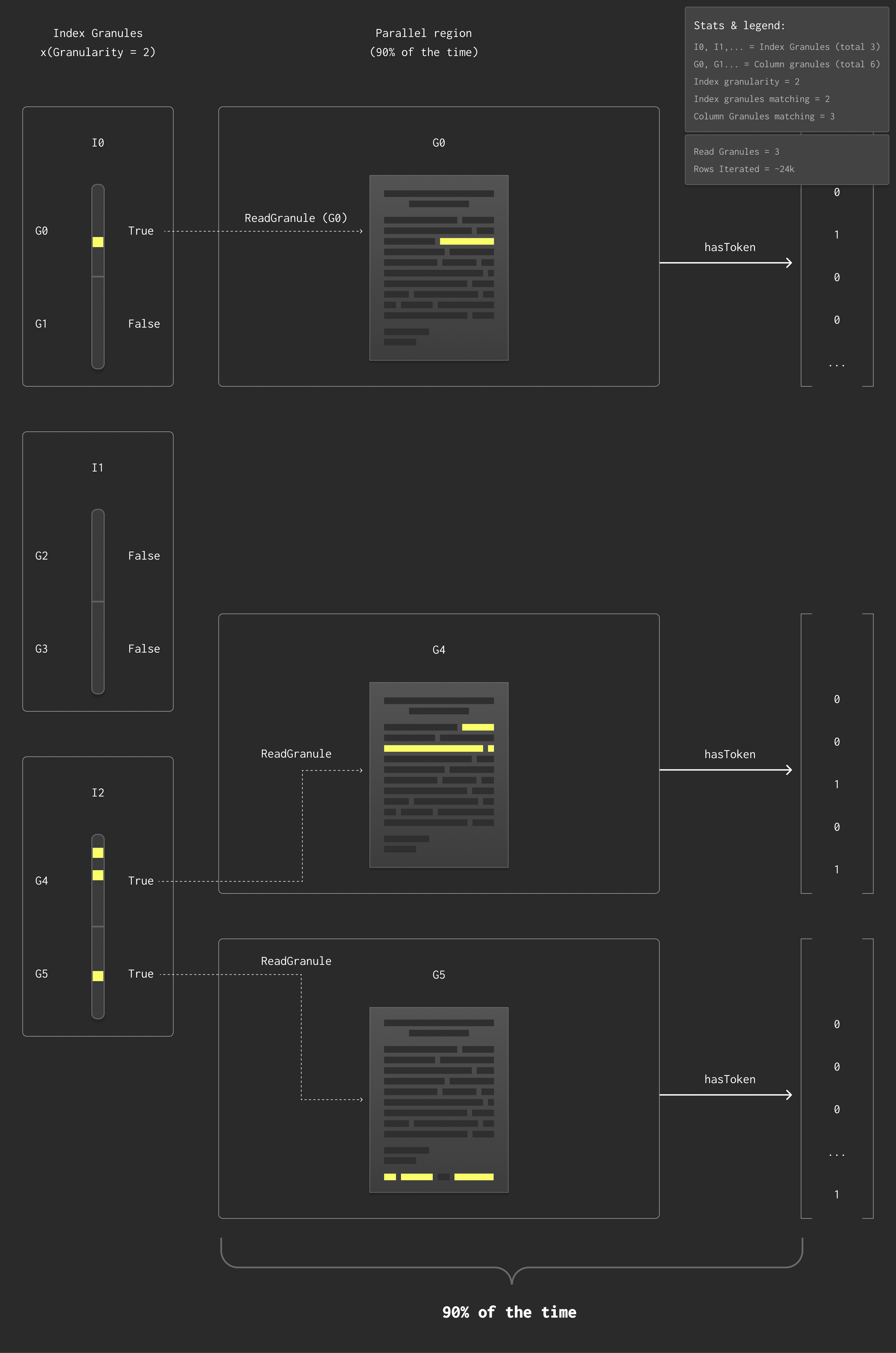
The next figure shows how we fixed this.

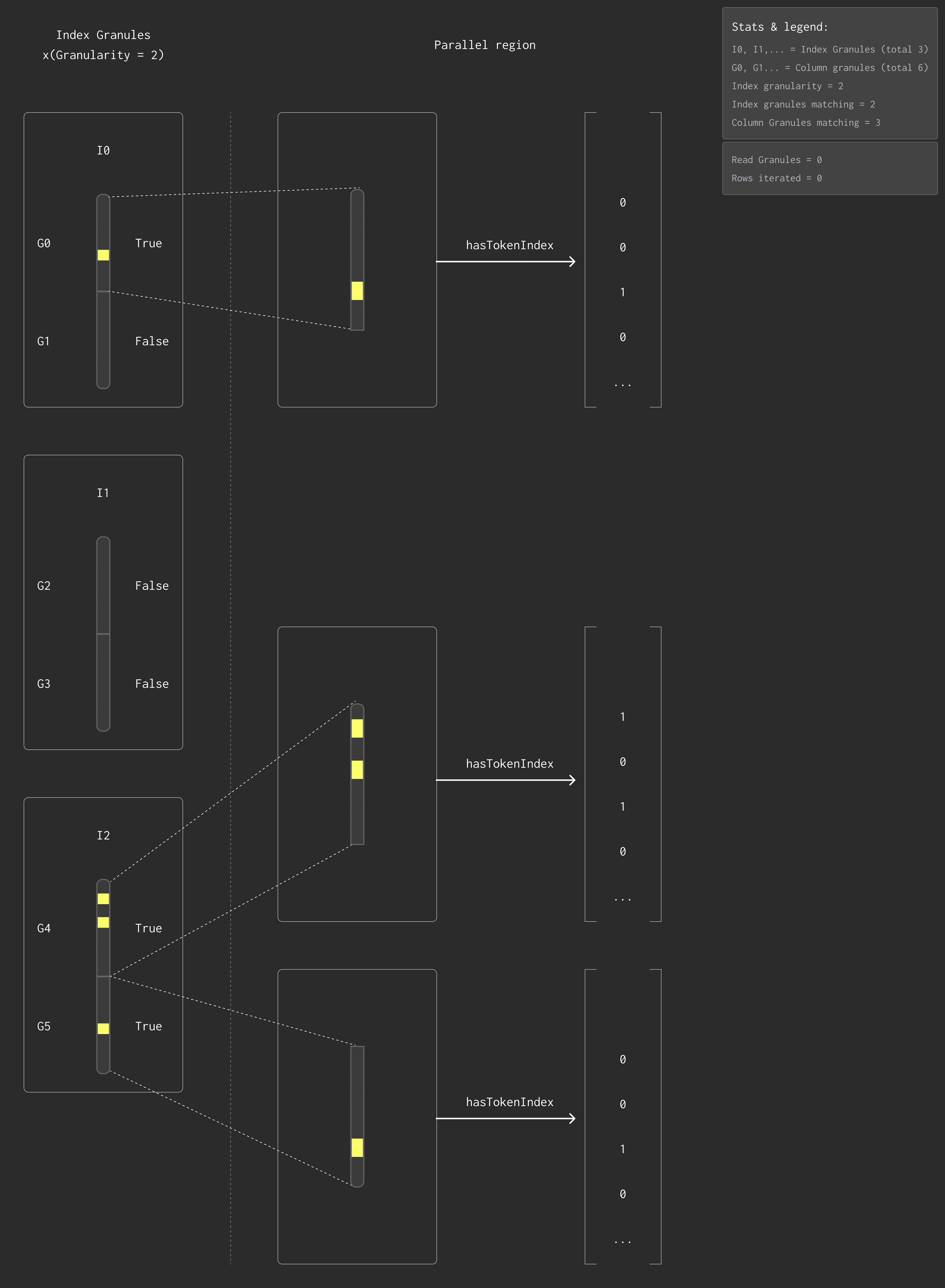
The new implementation filters entirely using the index — no text read required.

This removes the final bottleneck for full-text search performance.

Real-world gains #

We benchmarked this optimization using the Hacker News dataset (~27 million rows).

Tokens ranged from rare to very frequent:

Token frequency (%)	Previous implementation (sec)	Optimized cold run (sec)	Optimized hot run (sec)
90	1.6 - 2.2	0.43 - 0.6	0.026 - 0.06
50	1.4 - 2.0	0.18 - 0.3	0.03 - 0.05
~1	1.4 - 1.8	0.11 - 0.2	0.015 - 0.026
~0 (~10 matches)	0.2 - 0.5	0.11 - 0.15	0.008 - 0.012

(Benchmarks were run on an m6i.8xlarge instance (32 vCPUs, 128 GiB RAM, Xeon 8375C @ 3.5GHz))

Transparent to users #

This optimization is fully automatic, you don’t need to change your queries. We’re also continuing to improve cold-run performance and will make the feature generally available soon.

Together, these changes make ClickHouse’s full-text search faster and seamlessly integrated into your analytical workflows.

Your search ends here #

From tokenization to pure index access paths, the new native text index makes search in ClickHouse fast, precise, and fully integrated. With fuzzy matching, flexible analyzers, and row-level filtering that never touches the text column, you can run complex searches with the same efficiency as your analytical queries.

Built on months of engineering, tuning, and rethinking how full-text search should work in a column store, it’s now ready for you to put to the test.

You can now register for the private preview of the rebuilt full-text search, and we’re actively looking for early adopters to give feedback. Get early access and help shape what’s next.