
Introduction
We posted an article on Exploring massive, real-world data sets a few months ago, focusing on 100+ Years of Weather Records in ClickHouse. As we’ve recently enabled Dictionaries in ClickHouse Cloud, in this post, we’ll take the opportunity to remind users of the power of dictionaries for accelerating queries - especially those containing JOINs, as well as some usage tips.
Interested in trying dictionaries in ClickHouse Cloud? Get started instantly, with $300 free credit for 30 days.
In addition, all examples in this post can be reproduced in our play.clickhouse.com environment (see the blogs database). Alternatively, if you want to dive deeper into this dataset, ClickHouse Cloud is a great starting point - spin up a cluster using a free trial, load the data, let us deal with the infrastructure, and get querying!
A quick recap
For those of you new to the weather dataset, our original table schema looked like this:
CREATE TABLE noaa
(
   `station_id` LowCardinality(String),
   `date` Date32,
   `tempAvg` Int32 COMMENT 'Average temperature (tenths of a degrees C)',
   `tempMax` Int32 COMMENT 'Maximum temperature (tenths of degrees C)',
   `tempMin` Int32 COMMENT 'Minimum temperature (tenths of degrees C)',
   `precipitation` UInt32 COMMENT 'Precipitation (tenths of mm)',
   `snowfall` UInt32 COMMENT 'Snowfall (mm)',
   `snowDepth` UInt32 COMMENT 'Snow depth (mm)',
   `percentDailySun` UInt8 COMMENT 'Daily percent of possible sunshine (percent)',
   `averageWindSpeed` UInt32 COMMENT 'Average daily wind speed (tenths of meters per second)',
   `maxWindSpeed` UInt32 COMMENT 'Peak gust wind speed (tenths of meters per second)',
   `weatherType` Enum8('Normal' = 0, 'Fog' = 1, 'Heavy Fog' = 2, 'Thunder' = 3, 'Small Hail' = 4, 'Hail' = 5, 'Glaze' = 6, 'Dust/Ash' = 7, 'Smoke/Haze' = 8, 'Blowing/Drifting Snow' = 9, 'Tornado' = 10, 'High Winds' = 11, 'Blowing Spray' = 12, 'Mist' = 13, 'Drizzle' = 14, 'Freezing Drizzle' = 15, 'Rain' = 16, 'Freezing Rain' = 17, 'Snow' = 18, 'Unknown Precipitation' = 19, 'Ground Fog' = 21, 'Freezing Fog' = 22),
   `location` Point,
   `elevation` Float32,
   `name` LowCardinality(String)
) ENGINE = MergeTree() ORDER BY (station_id, date)
Each row represents measurements for a weather station at a point in time - a full description of the columns can be found in our original post. The original dataset had no notion of station name, elevation, or location, with each row having only a station_id. To keep queries simple, we originally de-normalized these onto each row from a stations.txt file to ensure every measurement had a geographical location and station name. Utilizing the fact that the first two digits of the station_id represent the country code, we can find the top 5 temperatures for a country by knowing its prefix and using the substring function. For example, Portugal:
SELECT tempMax / 10 AS maxTemp, station_id, date, location, name FROM noaa WHERE substring(station_id, 1, 2) = 'PO' ORDER BY tempMax DESC LIMIT 5 ┌─maxTemp─┬─station_id──┬───────date─┬─location──────────┬─name───────────┐ │ 45.8 │ PO000008549 │ 1944-07-30 │ (-8.4167,40.2) │ COIMBRA │ │ 45.4 │ PO000008562 │ 2003-08-01 │ (-7.8667,38.0167) │ BEJA │ │ 45.2 │ PO000008562 │ 1995-07-23 │ (-7.8667,38.0167) │ BEJA │ │ 44.5 │ POM00008558 │ 2003-08-01 │ (-7.9,38.533) │ EVORA/C. COORD │ │ 44.2 │ POM00008558 │ 2022-07-13 │ (-7.9,38.533) │ EVORA/C. COORD │ └─────────┴─────────────┴────────────┴───────────────────┴────────────────┘ 5 rows in set. Elapsed: 0.259 sec. Processed 1.08 billion rows, 7.46 GB (4.15 billion rows/s., 28.78 GB/s.)✎
This query, unfortunately requires a full table scan as it cannot exploit our primary key (station_id, date).
Improving the data model
Members of our community quickly proposed a simple optimization to improve the response time of the above query by reducing the amount of data read from disk. This can be achieved by skipping the denormalization and storing the station_id in a separate table before modifying the query to use a simple subquery.
Let's first recap this suggestion for the benefit of readers. Below we create a stations table and populate it directly by inserting the data over HTTP using a url function.
CREATE TABLE stations
(
    `station_id` LowCardinality(String),
    `country_code` LowCardinality(String),
    `state` LowCardinality(String),
    `name` LowCardinality(String),
    `lat` Float64,
    `lon` Float64,
    `elevation` Float32
)
ENGINE = MergeTree
ORDER BY (country_code, station_id)

INSERT INTO stations
SELECT
    station_id,
    substring(station_id, 1, 2) AS country_code,
    trimBoth(state) AS state,
    name,
    lat,
    lon,
    elevation
FROM url('https://noaa-ghcn-pds.s3.amazonaws.com/ghcnd-stations.txt', Regexp, 'station_id String, lat Float64, lon Float64, elevation Float32, state String, name String')
SETTINGS format_regexp = '^(.{11})\\s+(\\-?\\d{1,2}\\.\\d{4})\\s+(\\-?\\d{1,3}\\.\\d{1,4})\\s+(\\-?\\d*\\.\\d*)\\s+(.{2})\\s(.*?)\\s{2,}.*$'

0 rows in set. Elapsed: 1.781 sec. Processed 123.18 thousand rows, 7.99 MB (69.17 thousand rows/s., 4.48 MB/s.)
As noted in our original post, the stations.txt isn’t well formatted, so we use a Regex type to parse out the field values.
For example, we’ll now assume our noaa table no longer has a location, elevation, and name field. Our top 5 temperatures for Portugal query can now almost be solved with a subquery:
SELECT tempMax / 10 AS maxTemp, station_id, date, location, name FROM noaa WHERE station_id IN ( SELECT station_id FROM stations WHERE country_code = 'PO' ) ORDER BY tempMax DESC LIMIT 5 ┌─maxTemp─┬─station_id──┬───────date─┬─location──────────┬─name───────────┐ │ 45.8 │ PO000008549 │ 1944-07-30 │ (-8.4167,40.2) │ COIMBRA │ │ 45.4 │ PO000008562 │ 2003-08-01 │ (-7.8667,38.0167) │ BEJA │ │ 45.2 │ PO000008562 │ 1995-07-23 │ (-7.8667,38.0167) │ BEJA │ │ 44.5 │ POM00008558 │ 2003-08-01 │ (-7.9,38.533) │ EVORA/C. COORD │ │ 44.2 │ POM00008558 │ 2022-07-13 │ (-7.9,38.533) │ EVORA/C. COORD │ └─────────┴─────────────┴────────────┴───────────────────┴────────────────┘ 5 rows in set. Elapsed: 0.009 sec. Processed 522.48 thousand rows, 6.64 MB (59.81 million rows/s., 760.45 MB/s.)✎
This is faster as the subquery exploits the country_code primary key for the stations table. Furthermore, the parent query can also utilize its primary key. The need to only read smaller ranges of these columns, and thus less data off the disk, offsets any join cost. As pointed out by members of our community, keeping the data denormalized is beneficial in this case.
There is one issue here though - we are relying on the location and name being denormalized onto our weather data. If we assume we haven’t done this, to avoid de-duplication, and follow the principle of keeping it normalized and separate on the stations table we need a full join (in reality we would probably leave the location and name denormalized and accept the storage cost):
SELECT tempMax / 10 AS maxTemp, station_id, date, stations.name AS name, (stations.lat, stations.lon) AS location FROM noaa INNER JOIN stations ON noaa.station_id = stations.station_id WHERE stations.country_code = 'PO' ORDER BY tempMax DESC LIMIT 5 ┌─maxTemp─┬─station_id──┬───────date─┬─name───────────┬─location──────────┐ │ 45.8 │ PO000008549 │ 1944-07-30 │ COIMBRA │ (40.2,-8.4167) │ │ 45.4 │ PO000008562 │ 2003-08-01 │ BEJA │ (38.0167,-7.8667) │ │ 45.2 │ PO000008562 │ 1995-07-23 │ BEJA │ (38.0167,-7.8667) │ │ 44.5 │ POM00008558 │ 2003-08-01 │ EVORA/C. COORD │ (38.533,-7.9) │ │ 44.2 │ POM00008558 │ 2022-07-13 │ EVORA/C. COORD │ (38.533,-7.9) │ └─────────┴─────────────┴────────────┴────────────────┴───────────────────┘ 5 rows in set. Elapsed: 0.488 sec. Processed 1.08 billion rows, 14.06 GB (2.21 billion rows/s., 28.82 GB/s.)✎
This is unfortunately slower than our previous denormalized approach as it requires a full table scan. The reason for this can be found in our documentation.
When running a JOIN, there is no optimization of the order of execution in relation to other stages of the query. The join (a search in the right table) is run before filtering in WHERE and before aggregation.”
The documentation also suggests dictionaries as a possible solution. Let's now demonstrate how we can improve this query performance using a dictionary now that the data is normalized.
Creating a dictionary
Dictionaries provide us with an in-memory key-value pair representation of our data, optimized for low latent lookup queries. We can utilize this structure to improve the performance of queries in general, with JOINs particularly benefiting where one side of the JOIN represents a look-up table that fits into memory.
Choosing a source and key
In ClickHouse Cloud, the dictionary itself can currently be populated from two sources: local ClickHouse tables and HTTP URLs*. The dictionary's contents can then be configured to reload periodically to reflect any changes in the source data.
* We anticipate expanding this in the future to include support for other sources supported in OSS.
Below we create our dictionary using the stations table as the source.
CREATE DICTIONARY stations_dict
(
 `station_id` String,
 `state` String,
 `country_code` String,
 `name` String,
 `lat` Float64,
 `lon` Float64,
 `elevation` Float32
)
PRIMARY KEY station_id
SOURCE(CLICKHOUSE(TABLE 'stations'))
LIFETIME(MIN 0 MAX 0)
LAYOUT(complex_key_hashed_array())
The PRIMARY KEY here is the station_id and intuitively represents the column on which lookups will be performed. Values must be unique, i.e., rows with the same primary key will be deduplicated. The other columns represent attributes. You may notice that we have separated our location into lat and lon as the Point type is not currently supported as an attribute type for dictionaries. The LAYOUT and LIFETIME are less obvious and need some explanation.
Note: In ClickHouse Cloud, the dictionary will automatically be created on all nodes. For OSS, this behavior is possible if using a Replicated database. Other configurations will require the creation of the dictionary on all nodes manually or through the use of the ON CLUSTER clause.
Choosing a Layout
The layout of a dictionary controls how it is stored in memory and the indexing strategy for the primary key. Each of the layout options has different pros and cons.
The flat type allocates an array with as many entries as the largest key value, e.g., if the largest value is 100k, the array will also have 100k entries. This is well suited to cases where you have a monotonically increasing primary key in your source data. In this case, it is very memory-compact and provides access speeds 4-5x faster than the hash-based alternatives - a simple array offset lookup is required. However, it is limited in that the key size can also not exceed 500k - although this is configurable via the setting max_array_size. It is also inherently less efficient on large sparse distributions, wasting memory in such cases.
For cases where you have a very large number of entries, large key values, and/or a sparse distribution of values, then flat layout becomes less optimal. At this point, we would typically recommend a hash-based dictionary - specifically the hashed_array dictionary, which can efficiently support millions of entries. This layout is more memory efficient than the hashed layout and almost as fast. For this type, a hash table structure is used to store the primary key, with values providing offset positions into the attribute-specific arrays. This is in contrast hashed layout, which, although a little faster, requires a hash table to be allocated for each attribute - thus consuming more memory. In most cases, we, therefore, recommend the hashed_array layout - although users should experiment with hashed if they have only a few attributes.
All of these types also require the keys to be castable to UInt64. If not, e.g., they are Strings, we can use the complex variants of the hashed dictionaries: complex_key_hashed and complex_key_hashed_array, following the same rules above otherwise.
We try to capture the above logic with a flow chart below to help you choose the right layout (most of the time):
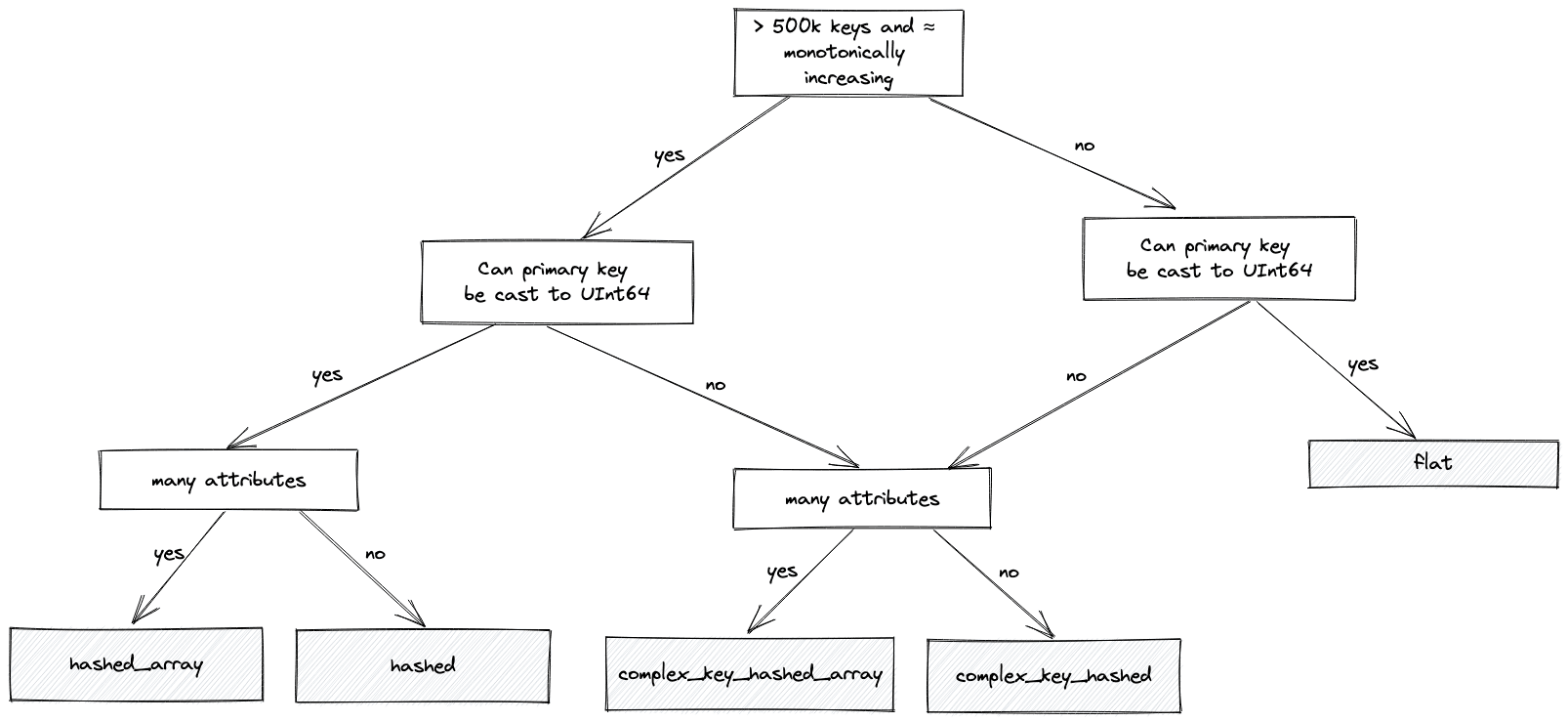
For our data, where our primary key is the String country_code, we choose the complex_key_hashed_array type since our dictionaries have at least three attributes in each case.
Note: We also have sparse variants of the hashed and complex_key_hashed layouts. This layout aims to achieve constant time operations by splitting the primary key into groups and incrementing a range within them. We rarely recommend this layout, which is only efficient if you have only one attribute. Although operations are constant time, the actual constant is typically higher than the non-sparse variants. Finally, ClickHouse offers specialized layouts such as polygon and ip_trie. We explored the former in the original blog, and will save others for future posts since they represent more advanced use cases.
Choosing a lifetime
Our above dictionary DDL also highlights the need to specify a LIFETIME for our dictionary. This specifies how often the dictionary should be refreshed by re-reading the source. This is specified in either seconds or as a range, e.g., LIFETIME(300) or LIFETIME(MIN 300 MAX 360). In the latter case, a value will choose a random time, uniformly distributed in the range. This ensures the load on the dictionary source is distributed over time when multiple servers are updating. The value LIFETIME(MIN 0 MAX 0), used in our example, means the dictionary contents will never be updated - appropriate in our case as our data is static.
If your data is changing and you need to reload the data periodically, this behavior can be controlled through an invalidate_query parameter which returns a row. If the value of this row changes between update cycles, ClickHouse knows the data must be re-fetched. This could, for example, return a timestamp or row count. Further options exist for ensuring only the data has changed since the previous update is loaded - see our documentation for examples of using the update_field.
Using a dictionary
Although our dictionary has been created, it requires a query to load the data into memory. The easiest ways to do this are to issue a simple dictGet query to retrieve a single value (loading the dataset into the dictionary as a by-product) or by issuing an explicit SYSTEM RELOAD DICTIONARY command.
SYSTEM RELOAD DICTIONARY stations_dict 0 rows in set. Elapsed: 0.561 sec. SELECT dictGet(stations_dict, 'state', 'CA00116HFF6') ┌─dictGet(stations_dict, 'state', 'CA00116HFF6')─┐ │ BC │ └────────────────────────────────────────────────┘ 1 row in set. Elapsed: 0.001 sec.✎
The dictGet example above retrieves the station_id value for the country code PO.
Returning to our original join query, we can restore our subquery and utilise the dictionary only for our location and name fields.
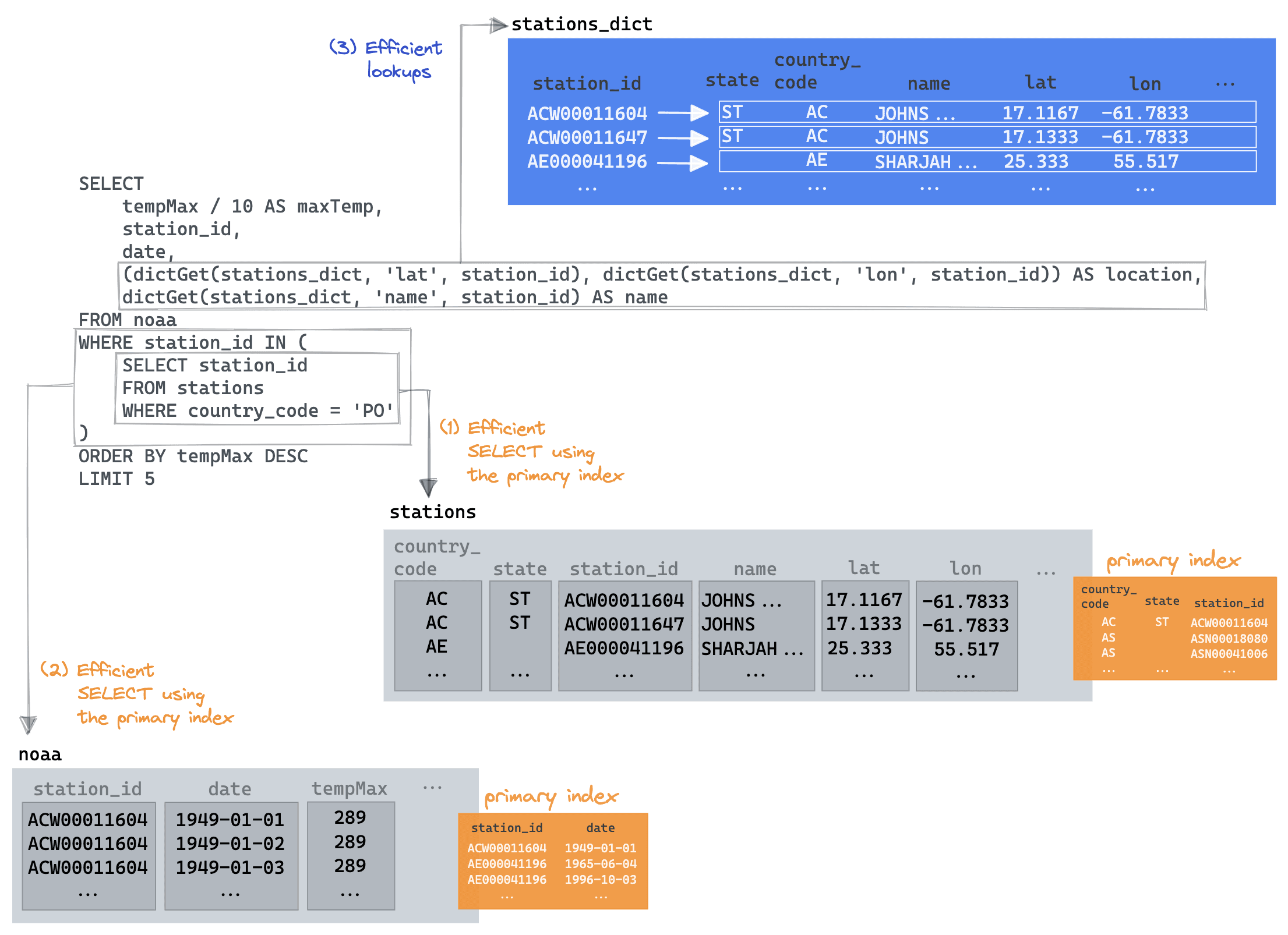
SELECT tempMax / 10 AS maxTemp, station_id, date, (dictGet(stations_dict, 'lat', station_id), dictGet(stations_dict, 'lon', station_id)) AS location, dictGet(stations_dict, 'name', station_id) AS name FROM noaa WHERE station_id IN ( SELECT station_id FROM stations WHERE country_code = 'PO' ) ORDER BY tempMax DESC LIMIT 5 ┌─maxTemp─┬─station_id──┬───────date─┬─location──────────┬─name───────────┐ │ 45.8 │ PO000008549 │ 1944-07-30 │ (40.2,-8.4167) │ COIMBRA │ │ 45.4 │ PO000008562 │ 2003-08-01 │ (38.0167,-7.8667) │ BEJA │ │ 45.2 │ PO000008562 │ 1995-07-23 │ (38.0167,-7.8667) │ BEJA │ │ 44.5 │ POM00008558 │ 2003-08-01 │ (38.533,-7.9) │ EVORA/C. COORD │ │ 44.2 │ POM00008558 │ 2022-07-13 │ (38.533,-7.9) │ EVORA/C. COORD │ └─────────┴─────────────┴────────────┴───────────────────┴────────────────┘ 5 rows in set. Elapsed: 0.012 sec. Processed 522.48 thousand rows, 6.64 MB (44.90 million rows/s., 570.83 MB/s.)✎
Now that's better! The key here is we are able to exploit the subquery optimization, benefiting from it utilizing its country_code primary key. The parent query is then able to restrict the noaa table read to only those returned station ids, again exploiting its primary key to minimize the data read. Finally, the dictGet is only needed for the final 5 rows to retrieve the name and location. We visualize this below:
An experienced dictionary user might be tempted to try other approaches here. We could, for example:
- Drop the sub-query and utilise a
dictGet(stations_dict, 'country_code', station_id) = 'PO'filter. This isn't faster (around 0.5s) as a dictionary look-up needs to be made for each station. We look at a similar example to this below. - Exploit the fact that dictionaries can be used in JOIN clauses like tables (see below). This suffers from the same challenge as the previous proposal, delivering comparable performance.
We of course welcome improvements!
Something more complex
Consider the final query in our original blog post:
Using a list of ski resorts in the united states and their respective locations, we join these against the top 1000 weather stations with the most snow in any month in the last 5 yrs. Sorting this join by geoDistance and restricting the results to those where the distance is less than 20km, we select the top result per resort and sort this by total snow. Note we also restrict resorts to those above 1800m, as a broad indicator of good skiing conditions.
SELECT
    resort_name,
    total_snow / 1000 AS total_snow_m,
    resort_location,
    month_year
FROM
(
    WITH resorts AS
        (
            SELECT
                resort_name,
                state,
                (lon, lat) AS resort_location,
                'US' AS code
            FROM url('https://gist.githubusercontent.com/Ewiseman/b251e5eaf70ca52a4b9b10dce9e635a4/raw/9f0100fe14169a058c451380edca3bda24d3f673/ski_resort_stats.csv', CSVWithNames)
        )
    SELECT
        resort_name,
        highest_snow.station_id,
        geoDistance(resort_location.1, resort_location.2, station_location.1, station_location.2) / 1000 AS distance_km,
        highest_snow.total_snow,
        resort_location,
        station_location,
        month_year
    FROM
    (
        SELECT
            sum(snowfall) AS total_snow,
            station_id,
            any(location) AS station_location,
            month_year,
            substring(station_id, 1, 2) AS code
        FROM noaa
        WHERE (date > '2017-01-01') AND (code = 'US') AND (elevation > 1800)
        GROUP BY
            station_id,
            toYYYYMM(date) AS month_year
        ORDER BY total_snow DESC
        LIMIT 1000
    ) AS highest_snow
    INNER JOIN resorts ON highest_snow.code = resorts.code
    WHERE distance_km < 20
    ORDER BY
        resort_name ASC,
        total_snow DESC
    LIMIT 1 BY
        resort_name,
        station_id
)
ORDER BY total_snow DESC
LIMIT 5
Before we optimize this with dictionaries, let's replace the CTE containing our resorts with an actual table. This ensures we have the data local to our ClickHouse cluster and can avoid the HTTP latency of fetching the resorts.
CREATE TABLE resorts
(
   `resort_name` LowCardinality(String),
   `state` LowCardinality(String),
   `lat` Nullable(Float64),
   `lon` Nullable(Float64),
   `code` LowCardinality(String)
)
ENGINE = MergeTree
ORDER BY state
When we populate this table, we also take the opportunity to align the state field with the stations table (we’ll use this later). The resorts use state names, while the stations use a state code. To ensure these are consistent, we can map the state name to a code when inserting it into the resorts table. This represents another opportunity to create a dictionary - based on an HTTP source this time.
CREATE DICTIONARY states ( `name` String, `code` String ) PRIMARY KEY name SOURCE(HTTP(URL 'https://gist.githubusercontent.com/gingerwizard/b0e7c190474c847fdf038e821692ce9c/raw/19fdac5a37e66f78d292bd8c0ee364ca7e6f9a57/states.csv' FORMAT 'CSVWithNames')) LIFETIME(MIN 0 MAX 0) LAYOUT(COMPLEX_KEY_HASHED_ARRAY()) SELECT * FROM states LIMIT 2 ┌─name─────────┬─code─┐ │ Pennsylvania │ PA │ │ North Dakota │ ND │ └──────────────┴──────┘ 2 rows in set. Elapsed: 0.001 sec.✎
At insert time, we can map our state name to a state code for the resorts using the dictGet function.
INSERT INTO resorts SELECT
    resort_name,
    dictGet(states, 'code', state) AS state,
    lat,
    lon,
    'US' AS code
FROM url('https://gist.githubusercontent.com/Ewiseman/b251e5eaf70ca52a4b9b10dce9e635a4/raw/9f0100fe14169a058c451380edca3bda24d3f673/ski_resort_stats.csv', CSVWithNames)

0 rows in set. Elapsed: 0.389 sec.
Our original query is now significantly more simple.
SELECT resort_name, total_snow / 1000 AS total_snow_m, resort_location, month_year FROM ( SELECT resort_name, highest_snow.station_id, geoDistance(lon, lat, station_location.1, station_location.2) / 1000 AS distance_km, highest_snow.total_snow, station_location, month_year, (lon, lat) AS resort_location FROM ( SELECT sum(snowfall) AS total_snow, station_id, any(location) AS station_location, month_year, substring(station_id, 1, 2) AS code FROM noaa WHERE (date > '2017-01-01') AND (code = 'US') AND (elevation > 1800) GROUP BY station_id, toYYYYMM(date) AS month_year ORDER BY total_snow DESC LIMIT 1000 ) AS highest_snow INNER JOIN resorts ON highest_snow.code = resorts.code WHERE distance_km < 20 ORDER BY resort_name ASC, total_snow DESC LIMIT 1 BY resort_name, station_id ) ORDER BY total_snow DESC LIMIT 5 ┌─resort_name──────────┬─total_snow_m─┬─resort_location─┬─month_year─┐ │ Sugar Bowl, CA │ 7.799 │ (-120.3,39.27) │ 201902 │ │ Donner Ski Ranch, CA │ 7.799 │ (-120.34,39.31) │ 201902 │ │ Boreal, CA │ 7.799 │ (-120.35,39.33) │ 201902 │ │ Homewood, CA │ 4.926 │ (-120.17,39.08) │ 201902 │ │ Alpine Meadows, CA │ 4.926 │ (-120.22,39.17) │ 201902 │ └──────────────────────┴──────────────┴─────────────────┴────────────┘ 5 rows in set. Elapsed: 0.673 sec. Processed 580.53 million rows, 4.85 GB (862.48 million rows/s., 7.21 GB/s.)✎
Note the execution time to see if we can improve this further. This query still assumes the location is denormalized onto our weather measurements. We can now read this field from our stations_dict dictionary. This will also conveniently allow us to obtain the station state and use this for our join with the resorts table instead of the code. This join is smaller and hopefully faster, i.e., rather than joining all stations with all US resorts, we limit to the resorts in the same state.
Our resorts table is actually quite small (364 entries). Although moving it to a dictionary is unlikely to deliver any real performance benefit to this query, it probably represents a sensible means of storing the data given its size. We select resort_name as our primary key as this must be unique, as noted earlier.
CREATE DICTIONARY resorts_dict
(
    `state` String,
    `resort_name` String,
    `lat` Nullable(Float64),
    `lon` Nullable(Float64)
)
PRIMARY KEY resort_name
SOURCE(CLICKHOUSE(TABLE 'resorts'))
LIFETIME(MIN 0 MAX 0)
LAYOUT(COMPLEX_KEY_HASHED_ARRAY())
Now let's make the changes to our query to use the stations_dict where possible and join on resorts_dict. Note how we still join on the state column even though it is not a primary key in our resorts dictionary. In this case, we use the JOIN syntax, and the dictionary will be scanned like a table.
SELECT resort_name, total_snow / 1000 AS total_snow_m, resort_location, month_year FROM ( SELECT resort_name, highest_snow.station_id, geoDistance(resorts_dict.lon, resorts_dict.lat, station_lon, station_lat) / 1000 AS distance_km, highest_snow.total_snow, (resorts_dict.lon, resorts_dict.lat) AS resort_location, month_year FROM ( SELECT sum(snowfall) AS total_snow, station_id, dictGet(stations_dict, 'lat', station_id) AS station_lat, dictGet(stations_dict, 'lon', station_id) AS station_lon, month_year, dictGet(stations_dict, 'state', station_id) AS state FROM noaa WHERE (date > '2017-01-01') AND (state != '') AND (elevation > 1800) GROUP BY station_id, toYYYYMM(date) AS month_year ORDER BY total_snow DESC LIMIT 1000 ) AS highest_snow INNER JOIN resorts_dict ON highest_snow.state = resorts_dict.state WHERE distance_km < 20 ORDER BY resort_name ASC, total_snow DESC LIMIT 1 BY resort_name, station_id ) ORDER BY total_snow DESC LIMIT 5 ┌─resort_name──────────┬─total_snow_m─┬─resort_location─┬─month_year─┐ │ Sugar Bowl, CA │ 7.799 │ (-120.3,39.27) │ 201902 │ │ Donner Ski Ranch, CA │ 7.799 │ (-120.34,39.31) │ 201902 │ │ Boreal, CA │ 7.799 │ (-120.35,39.33) │ 201902 │ │ Homewood, CA │ 4.926 │ (-120.17,39.08) │ 201902 │ │ Alpine Meadows, CA │ 4.926 │ (-120.22,39.17) │ 201902 │ └──────────────────────┴──────────────┴─────────────────┴────────────┘ 5 rows in set. Elapsed: 0.170 sec. Processed 580.73 million rows, 2.87 GB (3.41 billion rows/s., 16.81 GB/s.)✎
Nice, more than twice as fast! Now an astute reader will have noticed we skipped a possible optimization. Surely we could also replace our elevation check elevation > 1800 with a dictionary lookup for the value i.e. dictGet(blogs.stations_dict, 'elevation', station_id) > 1800, and thus avoid the table read? This will actually be slower as a dictionary lookup will be performed for every row, which is slower than evaluating the ordered elevation data - the latter benefits from the clause moving to PREWHERE. In this case, we benefit from elevation being denormalized. This is similar to how we didn’t use a dictGet in our earlier query to filter by country_code.
The advice here is thus to test! If dictGet is required for a large percentage of the rows in a table, e.g., in a condition, you may be better off just utilizing the native data structures and indexes of ClickHouse.
Final Tips
- The dictionary layouts we have described reside entirely in memory. Be mindful of their usage and test any layout changes. You can track their memory overhead using the system.dictionaries table and
bytes_allocatedcolumn. This table also includes alast_exceptioncolumn useful for diagnosing issues.
SELECT
    *,
    formatReadableSize(bytes_allocated) AS size
FROM system.dictionaries
LIMIT 1
FORMAT Vertical

Row 1:
──────
database:                           blogs
name:                               resorts_dict
uuid:                               0f387514-85ed-4c25-bebb-d85ade1e149f
status:                             LOADED
origin:                             0f387514-85ed-4c25-bebb-d85ade1e149f
type:                               ComplexHashedArray
key.names:                          ['resort_name']
key.types:                          ['String']
attribute.names:                    ['state','lat','lon']
attribute.types:                    ['String','Nullable(Float64)','Nullable(Float64)']
bytes_allocated:                    30052
hierarchical_index_bytes_allocated: 0
query_count:                        1820
hit_rate:                           1
found_rate:                         1
element_count:                      364
load_factor:                        0.7338709677419355
source:                             ClickHouse: blogs.resorts
lifetime_min:                       0
lifetime_max:                       0
loading_start_time:                 2022-11-22 16:26:06
last_successful_update_time:        2022-11-22 16:26:06
loading_duration:                   0.001
last_exception:
comment:
size:                               29.35 KiB
- While dictGet will likely be the dictionary function you use most, variants exist, with the dictGetOrDefault and dictHas being particularly useful. Also, note the type-specific functions e.g. dictGetFloat64
- The
flatdictionary size is limited to 500k entries. While this limit can be extended, consider it an indicator to move to a hashed layout. - For how Polygon dictionaries can be used to accelerate geo queries, we recommend our previous blog post.
Conclusion
In this blog post, we’ve demonstrated how keeping your data normalized can sometimes lead to faster queries, especially if using dictionaries. We’ve provided some simple and more complex examples of where dictionaries are valuable and concluded with some useful tips.
Acknowledgements
A special thanks to Stefan Käser for proposing improvements to our original post using Dictionaries to accelerate the queries.


