 50.5k
50.5k
A columnar database stores each column of a table together on disk, instead of storing each row together. That layout cuts I/O on analytical queries that touch a few columns from wide tables and lifts compression ratios into the 5–10× band (sometimes 30× on low-cardinality columns). ClickHouse, Snowflake, BigQuery, and DuckDB are columnar. Postgres and MySQL are row stores.
TL;DR
- Pick a columnar database when queries fit analytical patterns, like large time-range scans and aggregations. Pick a row store when point lookups and per-row writes are the primary pattern.
- Three multipliers compound: 5–10× compression, 90%+ I/O reduction on wide-table queries, and vectorised execution. Aggregations that take minutes on a row store finish in milliseconds on a columnar database.
- "Wide-column" databases like Cassandra and HBase are not the same as columnar databases. They are sparse-row key-value systems, not columnar OLAP engines.
What is a columnar database?
A columnar database is an OLAP-oriented system that stores each column of a table contiguously on disk, instead of storing each row together. The layout reduces I/O for queries that read a subset of columns and enables compression ratios of 5–10× (and up to 30× on low-cardinality columns) by grouping similar values together.
The idea predates the term. Copeland and Khoshafian formalised the decomposition storage model at SIGMOD 1985, splitting tables into per-attribute files. The production lineage starts with two 2005 papers. Stonebraker's C-Store at MIT was commercialised as Vertica. Boncz, Zukowski, and Nes's MonetDB/X100 at CWI defined the vectorised execution model that sits inside ClickHouse, DuckDB, Snowflake, Databricks Photon, Apache DataFusion, and Velox.
Columnar databases are sometimes called "column stores", and there's little distinction between the two terms. On the other hand, "columnar storage" refers specifcially to the layout of data on disk, and not the processing layer above it.
Benefits of columnar databases
- Efficient queries on subsets of columns — ideal for analytics, dashboards, and BI workloads.
- Fast aggregations on large datasets — scanning fewer columns reduces I/O and improves throughput.
- Better compression — similar values stored together compress much more effectively, reducing storage needs.
This makes columnar databases the preferred choice for analytical applications. They allow tables to have many columns without incurring a cost for unused columns at query time. Unlike traditional OLTP systems that always read entire rows, columnar systems are optimized for big data processing, data warehousing, and reporting use cases.
Modern columnar databases are designed to scale horizontally. ClickHouse, for example, combines real-time query performance with distributed scalability, making it well-suited for both traditional BI and real-time analytics use cases.
Row vs columnar databases
When a row-oriented database writes a record, it serialises every field — name, timestamp, price, region — into a single contiguous block on disk. Reading one complete row is fast because all the fields sit next to each other. But an analytical query that only needs the price column still has to scan past every other field in every row. At scale, this means reading orders of magnitude more data than the query actually requires.
Columnar databases flip the layout. Each column is stored in its own contiguous block: all the price values together, all the region values together, and so on. A query that aggregates prices touches only the price column and skips everything else. On a table with 50 columns, a query that reads 3 of them does roughly 6% of the I/O that a row store would need.
| Aspect | Row-oriented | Columnar |
|---|---|---|
| Storage layout | Tuples packed into pages | One file (or stripe) per column |
| Best workload | OLTP, single-row updates, point lookups | OLAP, aggregations, bulk scans |
| Compression | 1.5–3× typical | 5–10× typical, up to 30× |
| Read I/O on wide tables | Reads all columns | Reads only selected columns |
| Write path | Single-row insert/update in O(log n) | Bulk-append optimised; SQL UPDATE and DELETE supported |
| Concurrency | 1000s of point queries per node | 10s–100s of analytical queries per node |
| Examples | Postgres, MySQL, Oracle | ClickHouse, Snowflake, BigQuery |
In the row-based approach, all the values for a given row are adjacent, whereas in the column-based approach, the values for a given column are adjacent.
Here's how the two layouts compare at a glance:
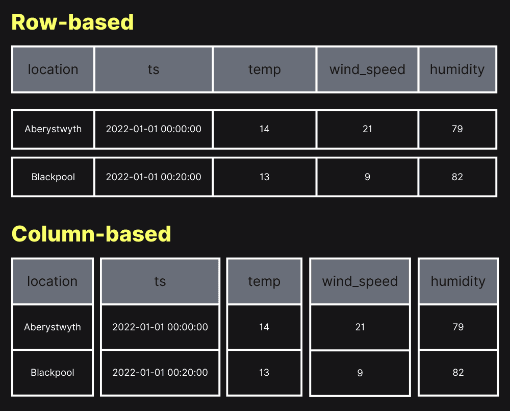
This layout also gives columnar databases an advantage in compression. Because adjacent values in a column share the same data type — and often similar magnitudes — encodings like dictionary encoding, run-length encoding, and delta encoding achieve compression ratios of 5–10× on real-world columnar data.
The tradeoff is writes. Inserting a single row means appending a value to every column file, which is more expensive than appending one contiguous block in a row store. Columnar databases handle this by batching writes into large chunks (often called "parts" or "row groups") and merging them in the background — a pattern that gives you high write throughput without sacrificing read performance.
Column storage is a fundamentally different physical layout that changes which operations are cheap and which are expensive. Row storage optimises for accessing complete records; columnar storage optimises for scanning and aggregating individual fields across large datasets.
When to pick which
Most organisations run both. A row-oriented RDBMS handles the application's transactional layer — user accounts, orders, inventory — where single-row reads and writes dominate and ACID guarantees matter. A columnar database sits behind the analytical layer (dashboards, reports, ad-hoc exploration), where queries scan millions of rows but typically touch only a handful of columns.
Change Data Capture (CDC) pipelines or tools like ClickPipes can replicate data from the transactional store into the columnar database in near-real-time, giving analysts fresh data without putting analytical load on the production database.
ClickHouse Cloud takes this a step further with its unified data stack: managed ClickHouse for analytics alongside managed PostgreSQL for transactions, with built-in replication between the two. Instead of stitching together separate services and CDC pipelines yourself, you get best-of-breed OLTP and OLAP in a single platform — PostgreSQL handles your application's transactional workload while ClickHouse handles the analytical workload, and data flows between them automatically.
Columnar database vs relational database
"Columnar" and "relational" describe different things, and the two aren't mutually exclusive. "Relational" refers to the data model — tables with rows, columns, primary keys, and joins. "Columnar" refers to the storage engine — how data is physically arranged on disk. A database can be both relational and columnar (ClickHouse uses SQL and supports joins, but stores data in columns), just as a database can be relational and row-oriented (PostgreSQL, MySQL).
In practice, when people search for "columnar database vs relational database" they usually mean columnar OLAP systems vs traditional row-oriented RDBMS.
When should I use a columnar database?
Use a columnar database when you want to run queries that aggregate and filter data across a few columns but lots of rows. These datasets will typically contain a lot of columns, but we’ll only be touching a subset of those columns in each query.
For example, take the real-world anonymized web analytics dataset that contains 100 million rows and has the following columns:
SELECT groupArray(name) AS columns
FROM system.columns
WHERE (database = 'metrica') AND (`table` = 'hits')
FORMAT Vertical;columns: ['WatchID','JavaEnable','Title','GoodEvent','EventTime','EventDate','CounterID','ClientIP','RegionID','UserID','CounterClass','OS','UserAgent','URL','Referer','Refresh','RefererCategoryID','RefererRegionID','URLCategoryID','URLRegionID','ResolutionWidth','ResolutionHeight','ResolutionDepth','FlashMajor','FlashMinor','FlashMinor2','NetMajor','NetMinor','UserAgentMajor','UserAgentMinor','CookieEnable','JavascriptEnable','IsMobile','MobilePhone','MobilePhoneModel','Params','IPNetworkID','TraficSourceID','SearchEngineID','SearchPhrase','AdvEngineID','IsArtifical','WindowClientWidth','WindowClientHeight','ClientTimeZone','ClientEventTime','SilverlightVersion1','SilverlightVersion2','SilverlightVersion3','SilverlightVersion4','PageCharset','CodeVersion','IsLink','IsDownload','IsNotBounce','FUniqID','OriginalURL','HID','IsOldCounter','IsEvent','IsParameter','DontCountHits','WithHash','HitColor','LocalEventTime','Age','Sex','Income','Interests','Robotness','RemoteIP','WindowName','OpenerName','HistoryLength','BrowserLanguage','BrowserCountry','SocialNetwork','SocialAction','HTTPError','SendTiming','DNSTiming','ConnectTiming','ResponseStartTiming','ResponseEndTiming','FetchTiming','SocialSourceNetworkID','SocialSourcePage','ParamPrice','ParamOrderID','ParamCurrency','ParamCurrencyID','OpenstatServiceName','OpenstatCampaignID','OpenstatAdID','OpenstatSourceID','UTMSource','UTMMedium','UTMCampaign','UTMContent','UTMTerm','FromTag','HasGCLID','RefererHash','URLHash','CLID']This table contains over 100 columns, but we’d usually consider only a few in each query. For example, we could write the following query to find the most popular mobile phone models in July 2013:
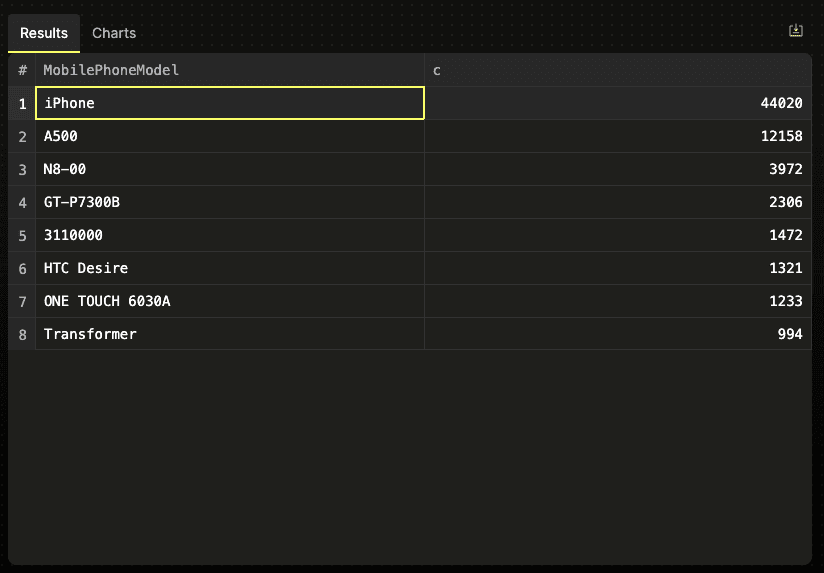
SELECT MobilePhoneModel, COUNT() AS c
FROM metrica.hits
WHERE
RegionID = 229
AND EventDate >= '2013-07-01'
AND EventDate <= '2013-07-31'
AND MobilePhone != 0
AND MobilePhoneModel not in ['', 'iPad']
GROUP BY MobilePhoneModel
ORDER BY c DESC
LIMIT 8;This query demonstrates several characteristics that make it ideal for a columnar database:
- Selective column access: Despite the table having over 100 columns, the query only needs to read data from
MobilePhoneModel,RegionID,EventDate, andMobilePhone. - Filtering: The
WHEREclause allows the database to eliminate irrelevant rows quickly. - Aggregation: The
COUNT()function aggregates data across millions of rows. - Large-scale processing: The query operates on a dataset of 100 million records, which is the lower bound of where column stores start showing their value for analytical queries.
You can try this query on the ClickHouse SQL Playground, hosted at sql.clickhouse.com.
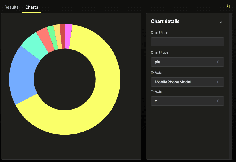
The query processes 100 million rows in under 100 milliseconds, and you can explore the results as a table:
Or as a chart:
When should I not use a columnar database?
While columnar databases excel in certain scenarios, particularly in analytical workloads involving large datasets, they are not a one-size-fits-all solution. Understanding their limitations is crucial for making informed decisions about database architecture.
Let's explore situations where there might be better choices than columnar databases.
Row-based lookups and OLTP workloads
Columnar databases are designed for analytics queries that typically aggregate or scan a few columns across many rows. However, they can be suboptimal for row-based lookups, common in Online Transaction Processing (OLTP) systems.
Consider our web analytics dataset example. If most of your queries resemble this:
SELECT *
FROM metrica.hits
WHERE WatchID = 8120543446287442873;A column store would need to:
- Read the
WatchIDcolumn to find the matching row - Fetch data from every other column for the matching row
- Reconstruct the full row(s)
This process can be inefficient, especially if you're fetching many columns. In contrast, a row-based store would have all the data for a single row stored contiguously, making such lookups much faster.
Real-world example: E-commerce platforms often need to retrieve all details of a specific order quickly. This operation is much more efficient in a row-based store.
Small datasets
The benefits of column stores become more apparent at scale. When dealing with smaller datasets (e.g., a few million rows or less), the performance difference between column and row stores for analytical queries might need to be more significant to justify adding another database.
For instance, if you're analyzing sales data for a small business with a few thousand monthly transactions, a well-indexed row-based database might perform satisfactorily without needing a column store.
Transactions
Most columnar databases don't support ACID (Atomicity, Consistency, Isolation, Durability) transactions, which are crucial for many business applications. If your use case requires strong transactional guarantees, a traditional row-based RDBMS would be a more suitable choice.
For instance, a banking system processing account transfers must ensure that debits and credits are applied atomically across accounts. This is typically easier to achieve with row-based, transactional databases.
What are popular column storage formats?
Many columnar databases use their own columnar storage format. But there are several columnar storage formats that are independent, such as Apache Parquet.
| Format | Description | Common Use Cases |
|---|---|---|
| Apache Parquet | Open-source, widely adopted columnar format with strong compression and encoding support. | Cloud data lakes, Spark, Presto/Trino, AWS Athena, Azure Synapse |
| Apache ORC (Optimized Row Columnar) | Designed for the Hadoop ecosystem - efficient storage for Hive and Spark workloads. | Hadoop/Hive environments, legacy big data pipelines |
| Apache Arrow** | An in-memory columnar format designed for fast analytics and data interchange. | DataFrames (e.g., Pandas, R), machine learning pipelines, cross-system data exchange |
These formats differ from full columnar databases like ClickHouse:
- File formats provide the on-disk storage representation.
- Databases add query execution, indexing, clustering, distribution, and more.
- Many columnar databases can query open formats directly (e.g., Parquet or ORC), but they also use their own optimized internal storage formats to achieve higher performance and feature integration.
Compression in columnar databases
Storing similar values adjacently lets columnar engines stack two compression layers. The encoding layer applies type-aware techniques: dictionary encoding for low-cardinality strings, run-length encoding for sorted runs, delta and delta-of-delta for monotonic sequences, Gorilla for floating-point time-series, and frame-of-reference plus bit-packing for residuals. A general-purpose codec (LZ4, ZSTD, or Snappy) compresses what the encodings leave behind. Typical ratios sit in the 5–10× band, with low-cardinality columns hitting 30× and above. Compression is one of the huge benefits of column stores, you can read more in the deep-dive on how columnar compression works.
What are the challenges of using a column store?
While column stores offer significant advantages for analytical workloads, they also present unique challenges, especially for users accustomed to traditional row-based systems. Understanding these challenges is crucial for effectively implementing and managing a column store database.
Updates
In row-based stores, updates are straightforward: data is modified in place, and the transaction is complete. However, column stores operate on a fundamentally different paradigm.
Column stores typically organize data into immutable column chunks. This immutability is a double-edged sword: it enables efficient compression and query performance but complicates the update process. The entire process becomes more intricate when a row needs to be updated.
We can’t update a row in place instead, we’ll need to write a new column chunk.
The column store's implementation will determine how the new value is made available to the query engine. The whole column chunk could be replaced, the new chunk could be merged with the existing one, or a lookup table may indicate the appropriate chunk to read for a given row.
This adds complexity to the database internals and means that column stores are generally optimized for inserting or updating records in larger batches rather than making many small updates.
However, modern column stores have made significant breakthroughs in update efficiency. ClickHouse, for example, introduced patch parts that treat updates as lightweight deltas rather than full column rewrites. Instead of rewriting entire chunks, patch parts contain only the changed values and apply them during background merges or query processing. This innovation enables standard SQL UPDATE syntax with performance improvements of up to 1,000× while maintaining instant visibility of changes.
Denormalization
Historically, column stores were optimized for read-heavy workloads and often lacked efficient join capabilities. This limitation led to a common practice: denormalizing data during ingestion.
Denormalization involves combining data from multiple tables into a single, wide table. While this approach can significantly boost query performance, it comes with trade-offs:
- Data redundancy: Denormalized data often contains duplicated information, increasing storage requirements.
- Update complexity: Changes to denormalized data may require updates across multiple rows or columns.
- Data consistency: Maintaining consistency across denormalized data can be challenging, especially in systems with frequent updates.
Modern column stores have improved their join performance, making extreme denormalization unnecessary. However, for maximum query performance, some level of denormalization is often still beneficial. The challenge lies in finding the right balance between normalization (for data integrity and ease of updates) and denormalization (for query performance).
Knowing your query patterns
In column stores, the physical organization of data can dramatically impact query performance. Understanding your query patterns before data ingestion is crucial.
Key considerations include:
- Sort keys: Choosing the right columns to sort by can significantly speed up range queries and joins.
- Partitioning: Effective data partitioning can enable query engines to skip large chunks of irrelevant data.
For example, sorting data primarily by date could yield substantial performance benefits if most queries filter on date ranges. However, if this isn't considered during initial data loading, achieving optimal performance may require a costly data reorganization process.
What are some examples of columnar databases in 2026?
Below is a summary of some of the most notable columnar databases:
| # | Database | Deployment | License | Latency tier | Primary use case |
|---|---|---|---|---|---|
| 1 | ClickHouse | Self-hosted + managed | Apache 2.0 | Sub-second | Real-time OLAP, customer-facing analytics, data warehousing |
| 2 | DuckDB | Embedded library | MIT | Sub-second | Single-user exploration of small files |
| 3 | Snowflake | Managed only | Commercial | Seconds to minutes | Traditional data warehousing |
| 4 | BigQuery | Managed only | Commercial | Seconds to minutes | Traditional data warehousing |
| 5 | Amazon Redshift | Managed only | Commercial | Seconds to minutes | Traditional data warehousing |
| 6 | Apache Druid | Self-hosted + managed | Apache 2.0 | Seconds | Customer-facing analytics |
| 7 | Apache Pinot | Self-hosted + managed | Apache 2.0 | Sub-second | Customer-facing analytics |
Frequently asked questions
Can I use row-based and column-based stores together?
Yes, this is quite common in hybrid architectures. Row-based stores handle OLTP (day-to-day transactional operations, real-time updates, ACID compliance) while column-based stores manage OLAP (large-scale analytics, analytical queries on historical data, read-heavy workloads). Organizations often use change data capture (CDC) techniques to keep these systems in sync.
How do column stores handle semi-structured data like JSON or logs?
Column stores handle semi-structured data in several ways: extracting frequently queried fields into dedicated columns (most efficient for analytics), storing raw text with parsing at query time (simpler but less efficient), or using native JSON support like ClickHouse’s JSON data type that provides JSON-specific functions for fast querying of nested fields. The approach depends on balancing ingestion ease with query performance.
Do column stores support concurrent writes at scale?
Yes, modern column stores like ClickHouse handle high write concurrency. Inserts create independent data parts that don't block each other or SELECT queries, with background merge processes consolidating parts without long locks. Features like asynchronous inserts batch small frequent events, and distributed setups can spread writes across replicas, with each replica supporting up to 1,000 concurrent queries.
Is ClickHouse a column database?
Yes, ClickHouse is a column database. It is available as open-source software and a cloud offering and is the fastest and most resource-efficient real-time data warehouse and open-source database.
ClickHouse Cloud is used by Sony, Lyft, Cisco, GitLab, and many others.
You can learn more about the problems that ClickHouse solves in the user stories section.
Why is ClickHouse a popular columnar database?
ClickHouse is widely adopted in 2026 because it delivers extremely fast analytical queries on large datasets while remaining efficient to operate. Its combination of real-time performance, distributed scalability, and open-source availability makes it a strong choice for organizations building both internal BI tools and external-facing analytics applications.
ClickHouse continues to evolve rapidly, with an active open-source community and a growing cloud service used by companies of all sizes.


