What is ClickHouse?

ClickHouse® is a high-performance, column-oriented SQL database management system (DBMS) for online analytical processing (OLAP). It is available as both an open-source software and a cloud offering.

What are analytics?

Analytics, also known as OLAP (Online Analytical Processing), refers to SQL queries with complex calculations (e.g., aggregations, string processing, arithmetic) over massive datasets. Unlike transactional queries (or OLTP, Online Transaction Processing) that read and write just a few rows per query and, therefore, complete in milliseconds, analytics queries routinely process billions and trillions of rows. In many use cases, analytics queries must be “real-time”, i.e., return a result in less than one second.

Row-oriented vs. column-oriented storage

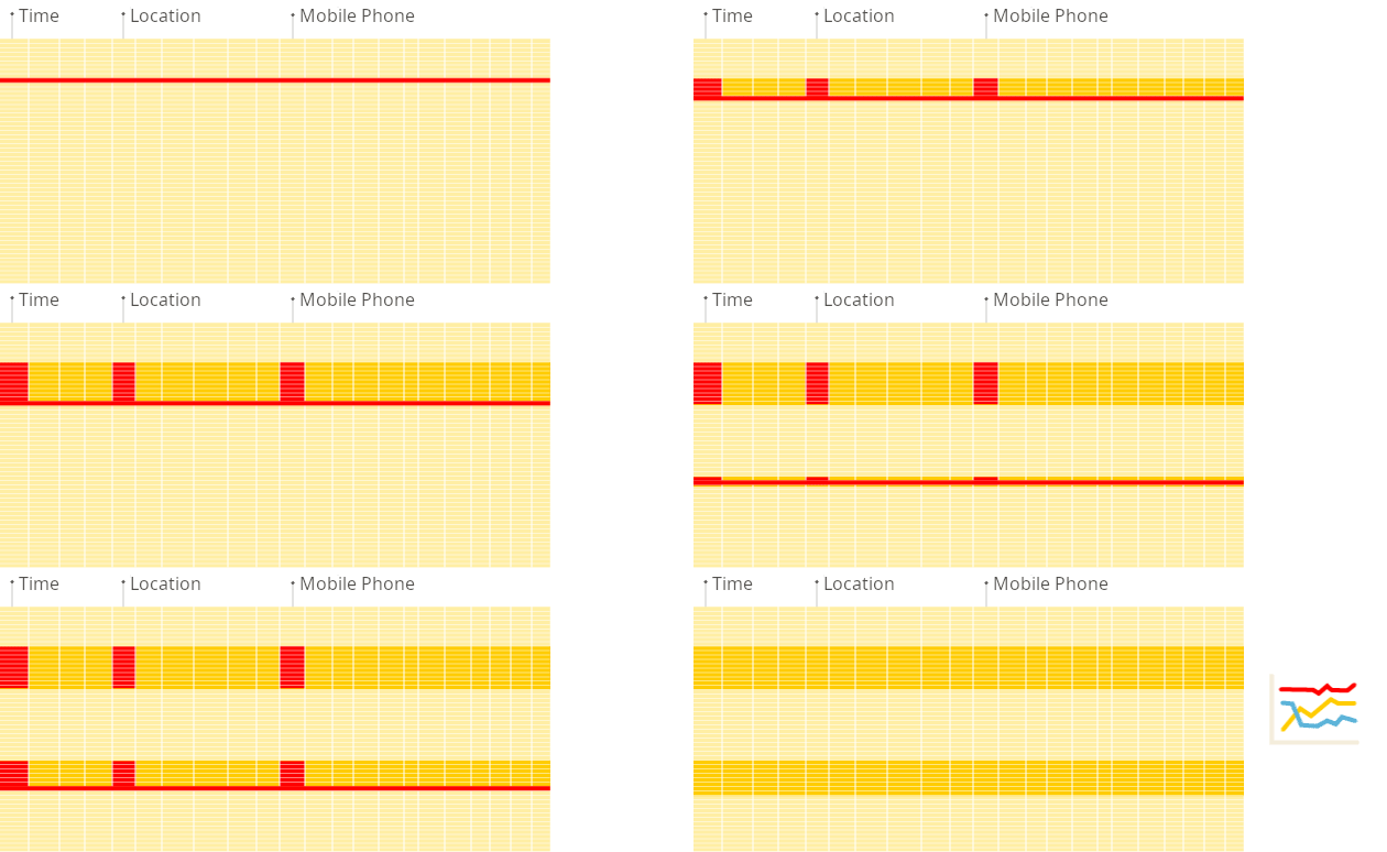
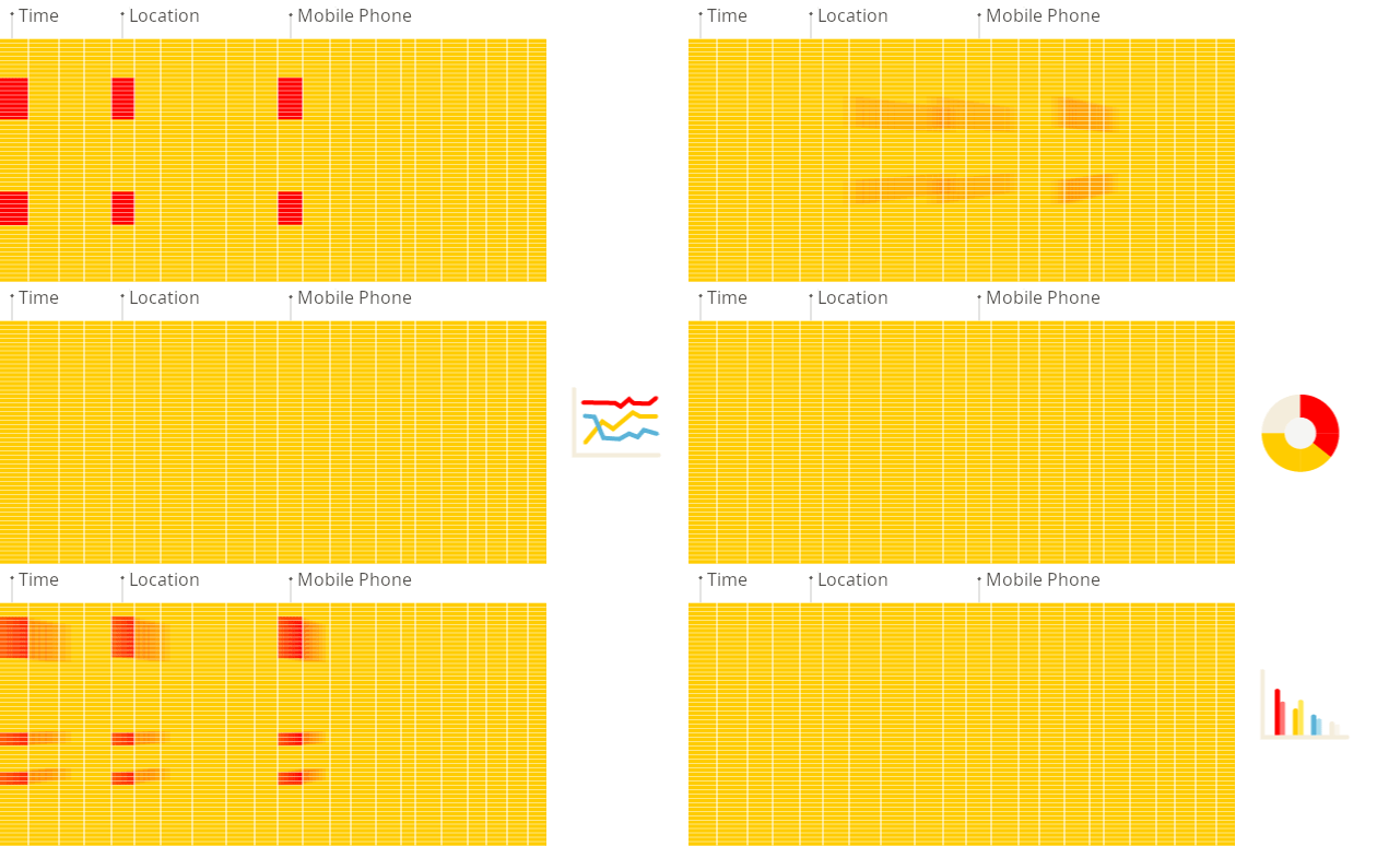
Such a level of performance can only be achieved with the right data “orientation”. Databases store data either row-oriented or column-oriented. In a row-oriented database, consecutive table rows are sequentially stored one after the other. This layout allows to retrieve rows quickly as the column values of each row are stored together. ClickHouse is a column-oriented database. In such systems, tables are stored as a collection of columns, i.e. the values of each column are stored sequentially one after the other. This layout makes it harder to restore single rows (as there are now gaps between the row values) but column operations such as filters or aggregation become much faster than in a row-oriented database. The difference is best explained with an example query running over 100 million rows of real-world anonymized web analytics data:

SELECT MobilePhoneModel, count() AS c
FROM metrica.hits
WHERE
      RegionID = 229
  AND EventDate >= '2013-07-01'
  AND EventDate <= '2013-07-31'
  AND MobilePhone != 0
  AND MobilePhoneModel NOT IN ('', 'iPad')
GROUP BY MobilePhoneModel
ORDER BY c DESC
LIMIT 8;

You can run this query on the ClickHouse SQL Playground that selects and filters just a few out of over 100 existing columns, returning the result within milliseconds:

Example query in a column-oriented database

As you can see in the stats section in the above diagram, the query processed 100 million rows in 92 milliseconds, a throughput of approximately over 1 billion rows per second or just under 7 GB of data transferred per second. Row-oriented DBMS In a row-oriented database, even though the query above only processes a few out of the existing columns, the system still needs to load the data from other existing columns from disk to memory. The reason for that is that data is stored on disk in chunks called blocks (usually fixed sizes, e.g., 4 KB or 8 KB). Blocks are the smallest units of data read from disk to memory. When an application or database requests data, the operating system’s disk I/O subsystem reads the required blocks from the disk. Even if only part of a block is needed, the entire block is read into memory (this is due to disk and file system design):

Column-oriented DBMS Because the values of each column are stored sequentially one after the other on disk, no unnecessary data is loaded when the query from above is run. Because the block-wise storage and transfer from disk to memory is aligned with the data access pattern of analytical queries, only the columns required for a query are read from disk, avoiding unnecessary I/O for unused data. This is much faster compared to row-based storage, where entire rows (including irrelevant columns) are read:

Data replication and integrity

ClickHouse uses an asynchronous multi-master replication scheme to ensure that data is stored redundantly on multiple nodes. After being written to any available replica, all the remaining replicas retrieve their copy in the background. The system maintains identical data on different replicas. Recovery after most failures is performed automatically, or semi-automatically in complex cases.

Role-Based Access Control

ClickHouse implements user account management using SQL queries and allows for role-based access control configuration similar to what can be found in ANSI SQL standard and popular relational database management systems.

SQL support

ClickHouse supports a declarative query language based on SQL that is identical to the ANSI SQL standard in many cases. Supported query clauses include GROUP BY, ORDER BY, subqueries in FROM, JOIN clause, IN operator, window functions and scalar subqueries.

Approximate calculation

ClickHouse provides ways to trade accuracy for performance. For example, some of its aggregate functions calculate the distinct value count, the median, and quantiles approximately. Also, queries can be run on a sample of the data to compute an approximate result quickly. Finally, aggregations can be run with a limited number of keys instead of for all keys. Depending on how skewed the distribution of the keys is, this can provide a reasonably accurate result that uses far fewer resources than an exact calculation.

Adaptive join algorithms

ClickHouse chooses the join algorithm adaptively: it starts with fast hash joins and falls back to merge joins if there’s more than one large table.

Superior query performance

ClickHouse is well known for having extremely fast query performance. To learn why ClickHouse is so fast, see the Why is ClickHouse fast? guide.

Get started

Setup

Sample datasets

Migrate