Optimizing ClickHouse with Schemas and Codecs

In this post, we’ll demonstrate the value of investing time in your ClickHouse schema through strict types and codecs to minimize your storage and improve your query performance.

For this purpose, we use a dataset from an earlier post: Exploring massive, real-world data sets: 100+ Years of Weather Records in ClickHouse. This dataset consists of rows, each describing weather measurements at a specific time and location for the last 100 years.

All examples in this post can be reproduced in our play.clickhouse.com environment (see the blogs database). Alternatively, if you want to dive deeper into this dataset, ClickHouse Cloud is a great solution - spin up a cluster using a free trial, load the data, let us deal with the infrastructure, and get querying!

A simplified version of this dataset’s schema is shown below; this is our starting schema.

CREATE TABLE noaa_codec_v1
(
   `station_id` String COMMENT 'Id of the station at which the measurement as taken',
   `date` Date32,
   `tempAvg` Int64 COMMENT 'Average temperature (tenths of a degrees C)',
   `tempMax` Int64 COMMENT 'Maximum temperature (tenths of degrees C)',
   `tempMin` Int64 COMMENT 'Minimum temperature (tenths of degrees C)',
   `precipitation` Int64 COMMENT 'Precipitation (tenths of mm)',
   `snowfall` Int64 COMMENT 'Snowfall (mm)',
   `snowDepth` Int64 COMMENT 'Snow depth (mm)',
   `percentDailySun` Int64 COMMENT 'Daily percent of possible sunshine (percent)',
   `averageWindSpeed` Int64 COMMENT 'Average daily wind speed (tenths of meters per second)',
   `maxWindSpeed` Int64 COMMENT 'Peak gust wind speed (tenths of meters per second)',
   `weatherType` String,
   `location` Point,
   `elevation` Float64,
   `name` String
) ENGINE = MergeTree() ORDER BY (station_id, date)

This is less optimized than the schema we used in our previous post - we’re deliberately using a poorer schema to show the benefit of being diligent concerning your types. We’ve selected this dataset as it contains a decent number and diversity of field types.

Our total dataset is around 1B rows. To assess the size of our data on the disk, we can use our system.columns table to compute the compression ratio of each column.

SELECT
    name,
    formatReadableSize(sum(data_compressed_bytes)) AS compressed_size,
    formatReadableSize(sum(data_uncompressed_bytes)) AS uncompressed_size,
    round(sum(data_uncompressed_bytes) / sum(data_compressed_bytes), 2) AS ratio
FROM system.columns
WHERE table = 'noaa_codec_v1'
GROUP BY name
ORDER BY sum(data_compressed_bytes) DESC

┌─name─────────────┬─compressed_size─┬─uncompressed_size─┬───ratio─┐
│ date             │ 2.24 GiB        │ 3.93 GiB          │    1.76 │
│ tempMax          │ 522.77 MiB      │ 7.87 GiB          │   15.41 │
│ tempMin          │ 519.53 MiB      │ 7.87 GiB          │   15.51 │
│ precipitation    │ 494.41 MiB      │ 7.87 GiB          │   16.29 │
│ tempAvg          │ 130.69 MiB      │ 7.87 GiB          │   61.64 │
│ snowDepth        │ 62.33 MiB       │ 7.87 GiB          │  129.26 │
│ weatherType      │ 37.87 MiB       │ 6.87 GiB          │   185.7 │
│ snowfall         │ 32.94 MiB       │ 7.87 GiB          │  244.56 │
│ location         │ 14.89 MiB       │ 15.73 GiB         │ 1081.94 │
│ averageWindSpeed │ 14.64 MiB       │ 7.87 GiB          │  550.29 │
│ maxWindSpeed     │ 11.09 MiB       │ 7.87 GiB          │  726.54 │
│ name             │ 9.63 MiB        │ 14.58 GiB         │ 1549.63 │
│ elevation        │ 7.95 MiB        │ 7.87 GiB          │ 1012.79 │
│ station_id       │ 7.60 MiB        │ 11.80 GiB         │ 1589.03 │
│ percentDailySun  │ 6.59 MiB        │ 7.87 GiB          │ 1222.67 │
└──────────────────┴─────────────────┴───────────────────┴─────────┘

15 rows in set. Elapsed: 0.005 sec.
 ✎

SELECT
    formatReadableSize(sum(data_compressed_bytes)) AS compressed_size,
    formatReadableSize(sum(data_uncompressed_bytes)) AS uncompressed_size,
    round(sum(data_uncompressed_bytes) / sum(data_compressed_bytes), 2) AS ratio
FROM system.columns
WHERE table = 'noaa_codec_v1'

┌─compressed_size─┬─uncompressed_size─┬─ratio─┐
│ 4.07 GiB        │ 131.58 GiB        │ 32.36 │
└─────────────────┴───────────────────┴───────┘

1 row in set. Elapsed: 0.004 sec.
 ✎

We’ll refer to these numbers throughout the blog and use these queries again to measure the impact of any schema changes we make. Ultimately we’re aiming to reduce both the uncompressed_size and compressed_size. This has a number of advantages beyond simply saving storage costs. Reduced data size on disk means less I/O at query time, potentially accelerating queries. While ClickHouse Cloud separates storage and compute, using object storage such as s3 also utilizes a local cache to reduce latency on queries that have similar access patterns. Higher compression means more data in the cache and more queries, potentially benefiting from not needing to download parts from the object store. The uncompressed_size is equally important to consider. Data must be decompressed prior to it being processed by queries. Larger data size post-decompression will result in greater RAM usage for query execution and potentially reduced CPU cache efficiency - both negatively impacting query performance.

An initial analysis of the compression ratio highlights how ClickHouse’s column-oriented design archives great compression out of the box, with no tuning, compressing this dataset thirty-two to one or over 96%*. We can, however, do better. Our initial focus should probably be on the largest columns, which currently have moderate compression: date, tempMax, tempMin, and precipitation.

*Note these measurements are taken in ClickHouse Cloud where ZSTD(1) is enabled by default (see below).

This sample query will be used before and after each of our changes to assess query performance. The following computes weather statistics for elevations every 100m. We don’t output any results as we’re ultimately interested in only the run time - hence FORMAT Null.

SELECT
    elevation_range,
    uniq(station_id) AS num_stations,
    max(tempMax) / 10 AS max_temp,
    min(tempMin) / 10 AS min_temp,
    sum(precipitation) AS total_precipitation,
    avg(percentDailySun) AS avg_percent_sunshine,
    max(maxWindSpeed) AS max_wind_speed,
    sum(snowfall) AS total_snowfall
FROM noaa_codec_v1
WHERE (date > '1970-01-01') AND (station_id IN (
    SELECT station_id
    FROM stations
    WHERE country_code = 'US'
))
GROUP BY floor(elevation, -2) AS elevation_range
ORDER BY elevation_range ASC
FORMAT `Null`

Ok.

0 rows in set. Elapsed: 1.615 sec. Processed 331.11 million rows, 23.19 GB (204.98 million rows/s., 14.36 GB/s.)
 ✎

Our first observation of the starting schema is that it uses unnecessary large bit representations for most integer fields. Let's identify the ranges of these fields and reduce our schema accordingly to use the appropriate integer length based on their supported ranges:

SELECT
    COLUMNS('Wind|temp|snow|pre') APPLY min,
    COLUMNS('Wind|temp|snow|pre') APPLY max
FROM blogs.noaa
FORMAT Vertical

Row 1:
──────
min(tempAvg):          -836
min(tempMax):          -830
min(tempMin):          -861
min(precipitation):    0
min(snowfall):         0
min(snowDepth):        0
min(averageWindSpeed): 0
min(maxWindSpeed):     0
max(tempAvg):          567
max(tempMax):          567
max(tempMin):          433
max(precipitation):    17500
max(snowfall):         1905
max(snowDepth):        11300
max(averageWindSpeed): 500
max(maxWindSpeed):     1131

1 row in set. Elapsed: 1.100 sec. Processed 1.08 billion rows, 34.46 GB (978.89 million rows/s., 31.32 GB/s.)
 ✎

CREATE TABLE noaa_codec_v2
(
  `station_id` String COMMENT 'Id of the station at which the measurement as taken',
  `date` Date32,
  `tempAvg` Int16 COMMENT 'Average temperature (tenths of a degrees C)',
  `tempMax` Int16 COMMENT 'Maximum temperature (tenths of degrees C)',
  `tempMin` Int16 COMMENT 'Minimum temperature (tenths of degrees C)',
  `precipitation` UInt16 COMMENT 'Precipitation (tenths of mm)',
  `snowfall` UInt16 COMMENT 'Snowfall (mm)',
  `snowDepth` UInt16 COMMENT 'Snow depth (mm)',
  `percentDailySun` UInt8 COMMENT 'Daily percent of possible sunshine (percent)',
  `averageWindSpeed` UInt16 COMMENT 'Average daily wind speed (tenths of meters per second)',
  `maxWindSpeed` UInt16 COMMENT 'Peak gust wind speed (tenths of meters per second)',
  `weatherType` String,
  `location` Point,
  `elevation` Int16,
  `name` String
) ENGINE = MergeTree() ORDER BY (station_id, date)

SELECT
    name,
    formatReadableSize(sum(data_compressed_bytes)) AS compressed_size,
    formatReadableSize(sum(data_uncompressed_bytes)) AS uncompressed_size,
    round(sum(data_uncompressed_bytes) / sum(data_compressed_bytes), 2) AS ratio
FROM system.columns
WHERE table = 'noaa_codec_v2'
GROUP BY name
ORDER BY sum(data_compressed_bytes) DESC

┌─name─────────────┬─compressed_size─┬─uncompressed_size─┬───ratio─┐
│ date             │ 2.23 GiB        │ 3.92 GiB          │    1.76 │
│ precipitation    │ 467.24 MiB      │ 1.96 GiB          │     4.3 │
│ tempMax          │ 449.87 MiB      │ 1.96 GiB          │    4.46 │
│ tempMin          │ 435.73 MiB      │ 1.96 GiB          │    4.61 │
│ tempAvg          │ 119.98 MiB      │ 1.96 GiB          │   16.74 │
│ snowDepth        │ 42.62 MiB       │ 1.96 GiB          │   47.11 │
│ weatherType      │ 37.72 MiB       │ 6.85 GiB          │  185.85 │
│ snowfall         │ 32.45 MiB       │ 1.96 GiB          │   61.87 │
│ location         │ 14.84 MiB       │ 15.69 GiB         │ 1082.21 │
│ averageWindSpeed │ 10.26 MiB       │ 1.96 GiB          │   195.8 │
│ name             │ 9.60 MiB        │ 14.53 GiB         │ 1549.76 │
│ station_id       │ 7.58 MiB        │ 11.77 GiB         │ 1589.08 │
│ maxWindSpeed     │ 6.29 MiB        │ 1.96 GiB          │  319.41 │
│ elevation        │ 1.88 MiB        │ 1.96 GiB          │  1066.4 │
│ percentDailySun  │ 1.51 MiB        │ 1004.00 MiB       │  666.23 │
└──────────────────┴─────────────────┴───────────────────┴─────────┘
✎

SELECT
    formatReadableSize(sum(data_compressed_bytes)) AS compressed_size,
    formatReadableSize(sum(data_uncompressed_bytes)) AS uncompressed_size,
    round(sum(data_uncompressed_bytes) / sum(data_compressed_bytes), 2) AS ratio
FROM system.columns
WHERE table = 'noaa_codec_v2'
┌─compressed_size─┬─uncompressed_size─┬─ratio─┐
│ 3.83 GiB        │ 71.38 GiB         │ 18.63 │
└─────────────────┴───────────────────┴───────┘
✎

The impact here is quite dramatic on the uncompressed_size, which has almost halved. This makes sense as we've reduced the integer precision and, thus, the number of bits required per value. Previous values, padded with significant zeros, obviously compressed well - our compressed_sizes are comparable. You may have also noticed the change in field type for the elevation field from Float64 to Int16. We may incur some precision loss here, but no likely analysis requires a precision greater than 1m with respect to elevation. This also saves us 6 GB of space when the data is uncompressed.

Before considering codecs, let's tidy up the String types. Our weather type can be represented by an Enum, reducing its representation from a variable string of N bytes to 8 bits per value. We can also dictionary encode our name and station_id columns using the LowCardinality super type. This type is usually effective to a cardinality of a few hundred thousand, but we always recommend testing. In our case, the fields have around 100k unique values.

Finally, our location field is costly at over 15GB uncompressed. This is due to the fact a Point type is represented as two Float64 values. Sampling our data and reviewing the original specification, we can see we don't have latitude and longitude values with greater precision than 5 decimal places. We can thus represent these as two Float32 fields. This will, however, mean that if we want to perform geo queries later, we might need to manually form a tuple at query time - the runtime cost here should be negligible.

CREATE TABLE noaa_codec_v3
(
 `station_id` LowCardinality(String) COMMENT 'Id of the station at which the measurement as taken',
 `date` Date32,
 `tempAvg` Int16 COMMENT 'Average temperature (tenths of a degrees C)',
 `tempMax` Int16 COMMENT 'Maximum temperature (tenths of degrees C)',
 `tempMin` Int16 COMMENT 'Minimum temperature (tenths of degrees C)',
 `precipitation` UInt16 COMMENT 'Precipitation (tenths of mm)',
 `snowfall` UInt16 COMMENT 'Snowfall (mm)',
 `snowDepth` UInt16 COMMENT 'Snow depth (mm)',
 `percentDailySun` UInt8 COMMENT 'Daily percent of possible sunshine (percent)',
 `averageWindSpeed` UInt16 COMMENT 'Average daily wind speed (tenths of meters per second)',
 `maxWindSpeed` UInt16 COMMENT 'Peak gust wind speed (tenths of meters per second)',
 `weatherType` Enum8('Normal' = 0, 'Fog' = 1, 'Heavy Fog' = 2, 'Thunder' = 3, 'Small Hail' = 4, 'Hail' = 5, 'Glaze' = 6, 'Dust/Ash' = 7, 'Smoke/Haze' = 8, 'Blowing/Drifting Snow' = 9, 'Tornado' = 10, 'High Winds' = 11, 'Blowing Spray' = 12, 'Mist' = 13, 'Drizzle' = 14, 'Freezing Drizzle' = 15, 'Rain' = 16, 'Freezing Rain' = 17, 'Snow' = 18, 'Unknown Precipitation' = 19, 'Ground Fog' = 21, 'Freezing Fog' = 22),
 `lat` Float32,
 `lon` Float32,
 `elevation` Int16,
 `name` LowCardinality(String)
) ENGINE = MergeTree() ORDER BY (station_id, date)

INSERT INTO noaa_codec_v3 SELECT station_id, date, tempAvg, tempMax, tempMin, precipitation, snowfall, snowDepth, percentDailySun, averageWindSpeed, maxWindSpeed, weatherType, location.2 as lat, location.1 as lon, elevation, name FROM noaa

SELECT
    name,
    formatReadableSize(sum(data_compressed_bytes)) AS compressed_size,
    formatReadableSize(sum(data_uncompressed_bytes)) AS uncompressed_size,
    round(sum(data_uncompressed_bytes) / sum(data_compressed_bytes), 2) AS ratio
FROM system.columns
WHERE table = 'noaa_codec_v3'
GROUP BY name
ORDER BY sum(data_compressed_bytes) DESC

┌─name─────────────┬─compressed_size─┬─uncompressed_size─┬───ratio─┐
│ date             │ 2.24 GiB        │ 3.94 GiB          │    1.76 │
│ precipitation    │ 469.11 MiB      │ 1.97 GiB          │     4.3 │
│ tempMax          │ 451.33 MiB      │ 1.97 GiB          │    4.47 │
│ tempMin          │ 437.15 MiB      │ 1.97 GiB          │    4.61 │
│ tempAvg          │ 120.28 MiB      │ 1.97 GiB          │   16.76 │
│ snowDepth        │ 42.80 MiB       │ 1.97 GiB          │    47.1 │
│ snowfall         │ 32.61 MiB       │ 1.97 GiB          │   61.81 │
│ weatherType      │ 16.48 MiB       │ 1008.00 MiB       │   61.16 │
│ averageWindSpeed │ 10.27 MiB       │ 1.97 GiB          │  196.24 │
│ maxWindSpeed     │ 6.31 MiB        │ 1.97 GiB          │  319.57 │
│ name             │ 3.99 MiB        │ 1.92 GiB          │  492.99 │
│ lat              │ 3.57 MiB        │ 3.94 GiB          │ 1127.84 │
│ lon              │ 3.57 MiB        │ 3.94 GiB          │ 1130.25 │
│ station_id       │ 3.40 MiB        │ 1.92 GiB          │   577.5 │
│ elevation        │ 1.89 MiB        │ 1.97 GiB          │ 1065.35 │
│ percentDailySun  │ 1.51 MiB        │ 1008.00 MiB       │  667.67 │
└──────────────────┴─────────────────┴───────────────────┴─────────┘
✎

SELECT
    formatReadableSize(sum(data_compressed_bytes)) AS compressed_size,
    formatReadableSize(sum(data_uncompressed_bytes)) AS uncompressed_size,
    round(sum(data_uncompressed_bytes) / sum(data_compressed_bytes), 2) AS ratio
FROM system.columns
WHERE table = 'noaa_codec_v3'

┌─compressed_size─┬─uncompressed_size─┬─ratio─┐
│ 3.81 GiB        │ 35.34 GiB         │  9.28 │
└─────────────────┴───────────────────┴───────┘
✎

Nice! we’ve halved our uncompressed size again, obtaining significant gains on the location (-50%), weatherType (-85%), and String columns especially. We also tested FixedString(11) for station_id, but it offered inferior performance (7.55 MiB compressed, 10.92 GiB uncompressed). Now let's evaluate our original query performance.

SELECT
    elevation_range,
    uniq(station_id) AS num_stations,
    max(tempMax) / 10 AS max_temp,
    min(tempMin) / 10 AS min_temp,
    sum(precipitation) AS total_precipitation,
    avg(percentDailySun) AS avg_percent_sunshine,
    max(maxWindSpeed) AS max_wind_speed,
    sum(snowfall) AS total_snowfall
FROM noaa_codec_v3
WHERE (date > '1970-01-01') AND (station_id IN (
    SELECT station_id
    FROM blogs.stations
    WHERE country_code = 'US'
))
GROUP BY floor(elevation, -2) AS elevation_range
ORDER BY elevation_range ASC
Format Null

0 rows in set. Elapsed: 1.132 sec. Processed 330.29 million rows, 6.39 GB (291.78 million rows/s., 5.64 GB/s.)
 ✎

With some trivial changes and diligence concerning our types, we’ve reduced our data size uncompressed from 134GB to 35GB.

Up to now, we’ve only performed type changes. With Column Compression Codecs, however, we can change the algorithm (and its settings) used to encode and compress each column.

Encoding and compression work slightly differently with the same objective: to reduce our data size. Encodings apply a mapping to our data, transforming the values based on a function by exploiting properties of the data type. Conversely, compression uses a generic algorithm to compress data at a byte level.

Typically, encodings are applied first before compression is used. Since different encodings and compression algorithms are effective on different value distributions, we must understand our data.

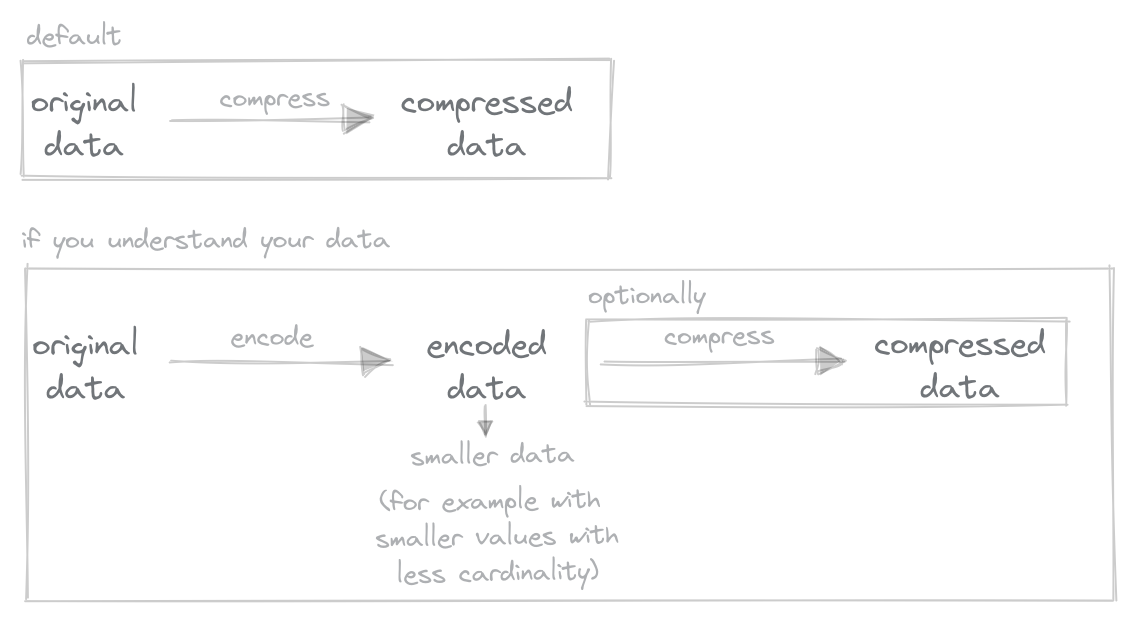
In ClickHouse Cloud, we utilize the ZSTD compression algorithm (with a default value of 1) by default. While compression speeds can vary for this algorithm, depending on the compression level (higher = slower), it has the advantage of being consistently fast on decompression (around 20% variance) and also benefiting from the ability to be parallelized. Our historical tests also suggest that this algorithm is often sufficiently effective and can even outperform LZ4 combined with a codec. It is effective on most data types, and information distributions and thus is a sensible general-purpose default and why our initial earlier compression is already excellent. In our results below, this value is represented as “DEFAULT(ZSTD)”.

If we understand our data, however, we can try to utilize more specialized codecs before also possibly applying a compressing algorithm. Delta compression works well on slowly changing numerics by replacing two neighboring values with their difference (except for the first value which stays unchanged). This generates a smaller number which requires fewer bits for storage. DoubleDelta takes the 2nd derivative. This can be particularly effective when the first delta is large and constant, e.g., dates at periodic intervals.

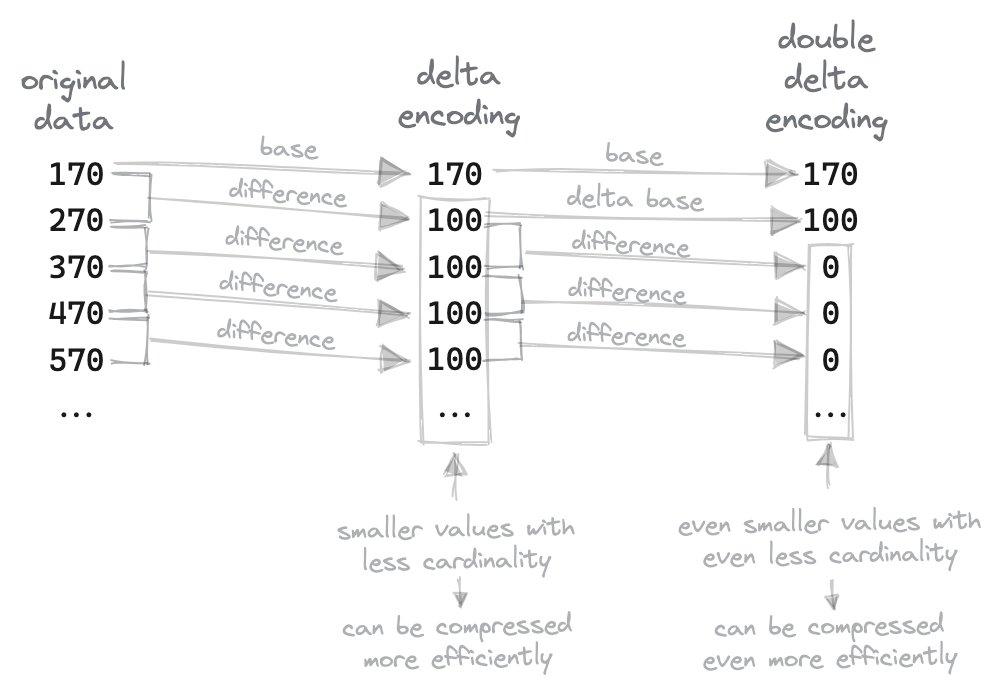
Given that our data is sorted by station_id and date (our primary keys), our measurements, such as temperature, should, in theory, change slowly, i.e., with the exception of the rare case of an extreme weather event, the derivative of the daily change in measurements such as snow, precipitation and temperature should be small. Below we apply Delta compression to our integer measurement fields. You’ll also notice that we also still apply ZSTD compression to our measurement fields - CODEC(Delta, ZSTD) utilizes a pipeline to encode the data first and then compresses the result. Delta encoding typically improves ZSTD, and this combination is common.

Finally, you’ll note that we also compress our Date field using the same technique. Date32 is a UInt32 and should have a constant interval of 1 day for most stations. They also haven’t compressed very well with plain ZSTD in our previous configurations, consuming 2.2GB and 60% of our compressed size.

CREATE TABLE noaa_codec_v4
(
    `station_id` LowCardinality(String),
    `date` Date32 CODEC(Delta, ZSTD),
    `tempAvg` Int16 CODEC(Delta, ZSTD),
    `tempMax` Int16 CODEC(Delta, ZSTD),
    `tempMin` Int16 CODEC(Delta, ZSTD),
    `precipitation` UInt16 CODEC(Delta, ZSTD),
    `snowfall` UInt16 CODEC(Delta, ZSTD),
    `snowDepth` UInt16 CODEC(Delta, ZSTD),
    `percentDailySun` UInt8 CODEC(Delta, ZSTD),
    `averageWindSpeed` UInt16 CODEC(Delta, ZSTD),
    `maxWindSpeed` UInt16 CODEC(Delta, ZSTD),
    `weatherType` Enum8('Normal' = 0, 'Fog' = 1, 'Heavy Fog' = 2, 'Thunder' = 3, 'Small Hail' = 4, 'Hail' = 5, 'Glaze' = 6, 'Dust/Ash' = 7, 'Smoke/Haze' = 8, 'Blowing/Drifting Snow' = 9, 'Tornado' = 10, 'High Winds' = 11, 'Blowing Spray' = 12, 'Mist' = 13, 'Drizzle' = 14, 'Freezing Drizzle' = 15, 'Rain' = 16, 'Freezing Rain' = 17, 'Snow' = 18, 'Unknown Precipitation' = 19, 'Ground Fog' = 21, 'Freezing Fog' = 22),
    `lat` Float32,
    `lon` Float32,
    `elevation` Int16,
    `name` LowCardinality(String)
)
ENGINE = MergeTree
ORDER BY (station_id, date)

INSERT INTO noaa_codec_v4 SELECT station_id, date, tempAvg, tempMax, tempMin, precipitation, snowfall, snowDepth, percentDailySun, averageWindSpeed, maxWindSpeed, weatherType, location.2 as lat, location.1 as lon, elevation, name FROM noaa

SELECT
    name,
    formatReadableSize(sum(data_compressed_bytes)) AS compressed_size,
    formatReadableSize(sum(data_uncompressed_bytes)) AS uncompressed_size,
    round(sum(data_uncompressed_bytes) / sum(data_compressed_bytes), 2) AS ratio
FROM system.columns
WHERE table = 'noaa_codec_v4'
GROUP BY name
ORDER BY sum(data_compressed_bytes) DESC

┌─name─────────────┬─compressed_size─┬─uncompressed_size─┬───ratio─┐
│ precipitation    │ 604.01 MiB      │ 1.99 GiB          │    3.38 │
│ tempMax          │ 451.59 MiB      │ 1.99 GiB          │    4.52 │
│ tempMin          │ 443.79 MiB      │ 1.99 GiB          │     4.6 │
│ tempAvg          │ 111.47 MiB      │ 1.99 GiB          │    18.3 │
│ snowDepth        │ 44.88 MiB       │ 1.99 GiB          │   45.45 │
│ snowfall         │ 42.50 MiB       │ 1.99 GiB          │      48 │
│ date             │ 24.55 MiB       │ 3.98 GiB          │  166.18 │
│ weatherType      │ 16.73 MiB       │ 1020.00 MiB       │   60.96 │
│ averageWindSpeed │ 12.28 MiB       │ 1.99 GiB          │  166.14 │
│ maxWindSpeed     │ 8.38 MiB        │ 1.99 GiB          │  243.41 │
│ name             │ 4.11 MiB        │ 1.94 GiB          │  482.25 │
│ lat              │ 3.62 MiB        │ 3.98 GiB          │ 1127.58 │
│ lon              │ 3.61 MiB        │ 3.98 GiB          │ 1129.96 │
│ station_id       │ 3.53 MiB        │ 1.94 GiB          │  561.62 │
│ percentDailySun  │ 2.01 MiB        │ 1020.00 MiB       │  507.31 │
│ elevation        │ 1.92 MiB        │ 1.99 GiB          │ 1065.16 │
└──────────────────┴─────────────────┴───────────────────┴─────────┘

16 rows in set. Elapsed: 0.007 sec.
✎

SELECT
    formatReadableSize(sum(data_compressed_bytes)) AS compressed_size,
    formatReadableSize(sum(data_uncompressed_bytes)) AS uncompressed_size,
    sum(data_uncompressed_bytes) / sum(data_compressed_bytes) AS compression_ratio
FROM system.columns
WHERE table = 'noaa_codec_v4'

┌─compressed_size─┬─uncompressed_size─┬─compression_ratio─┐
│ 1.74 GiB        │ 35.75 GiB         │ 20.57648186922219 │
└─────────────────┴───────────────────┴───────────────────┘

1 row in set. Elapsed: 0.005 sec.
✎

Nice, we’ve reduced our compressed size by over half. However, this is nearly entirely attributed to the reduction in the date field, which has reduced to 22.41MB! (this is effective as our intervals of 1 day reduce our data size to a single digit). The compression ratio of other columns haven’t improved and, in some cases, worsened, e.g., precipitation. This is initially surprising but can be largely attributed to data sparsity (and the effectiveness of plain ZSTD!), with a large number of 0s for many columns, i.e., many stations only make one or two measurements.

SELECT
    countIf(precipitation = 0) AS num_empty,
    countIf(precipitation > 0) AS num_non_zero,
    num_empty / (num_empty + num_non_zero) AS ratio
FROM noaa

┌─num_empty─┬─num_non_zero─┬──────────────ratio─┐
│ 792201587 │    284680862 │ 0.7356435121917378 │

└───────────┴──────────────┴────────────────────┘

SELECT
    countIf(snowDepth = 0) AS num_empty,
    countIf(snowDepth > 0) AS num_non_zero,
    num_empty / (num_empty + num_non_zero) AS ratio
FROM noaa

┌──num_empty─┬─num_non_zero─┬──────────────ratio─┐
│ 1032675925 │     44206524 │ 0.9589495361902773 │
└────────────┴──────────────┴────────────────────┘

SELECT
    countIf(maxWindSpeed = 0) AS num_empty,
    countIf(maxWindSpeed > 0) AS num_non_zero,
    num_empty / (num_empty + num_non_zero) AS ratio
FROM noaa

┌──num_empty─┬─num_non_zero─┬────────────ratio─┐
│ 1071299364 │      5583085 │ 0.99481551119606 │
└────────────┴──────────────┴──────────────────┘

(similar to tempMin) 
SELECT
    countIf(tempMax = 0) AS num_empty,
    countIf(tempMax > 0) AS num_non_zero,
    num_empty / (num_empty + num_non_zero) AS ratio
FROM noaa

┌─num_empty─┬─num_non_zero─┬──────────────ratio─┐
│ 639614575 │    396462468 │ 0.6173426767067167 │
└───────────┴──────────────┴────────────────────┘
 ✎

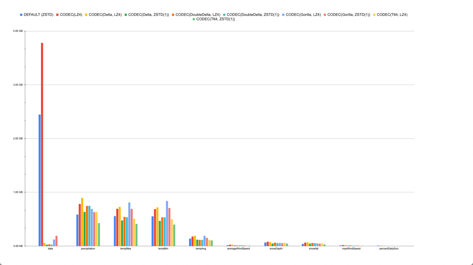
At this point, we decided to try the other encodings supported for integers. Below we show the values for Gorilla, DoubleDelta, and T64. We also test how effective these are with LZ4 and ZSTD compression.

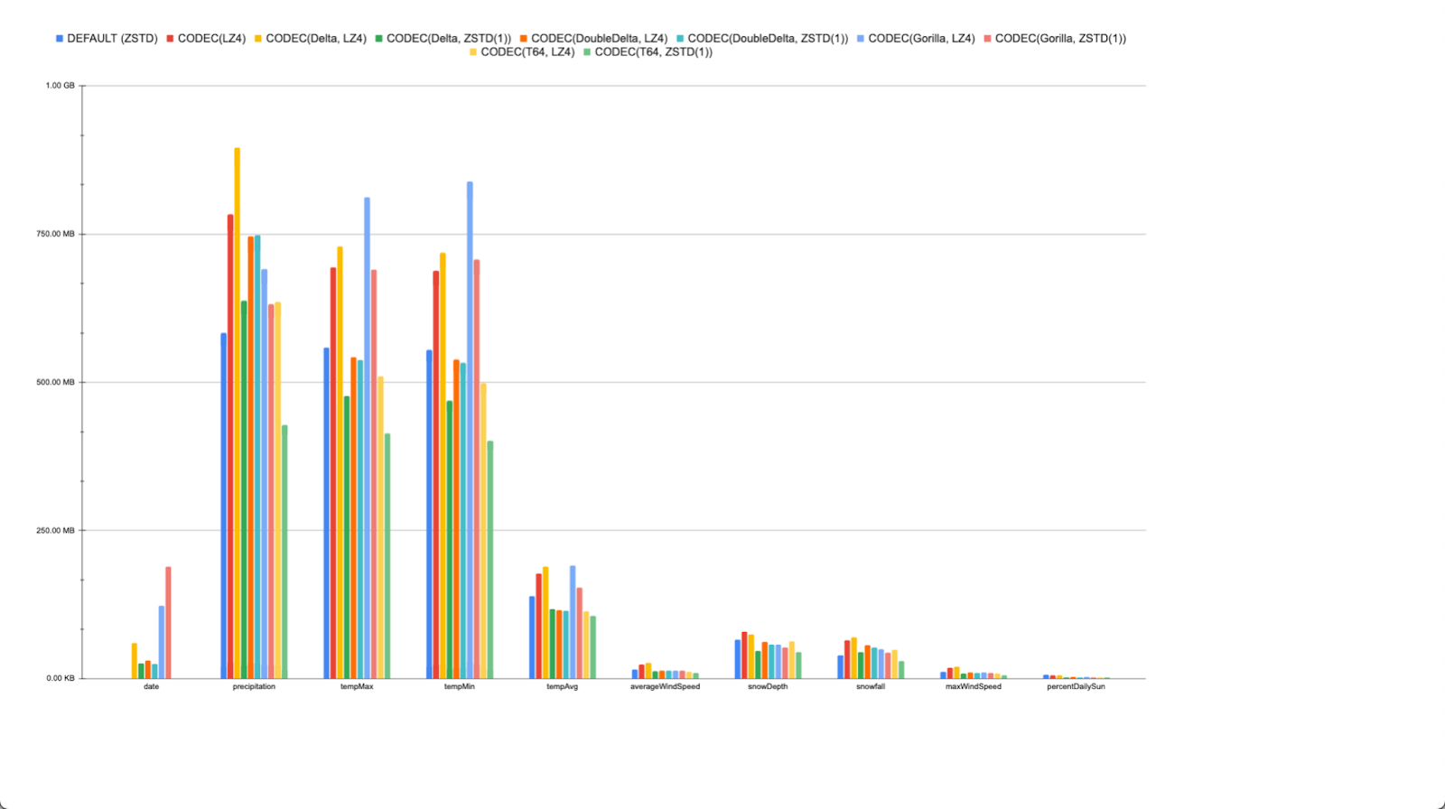
The date values, with no codec, obviously make this challenging to read. Removing these values provides a clearer indication of the effective codecs.

What's immediately apparent is that none of the codecs give us dramatic savings (date aside), but T64, when compressed with ZSTD tends to effectively reduce the size by around 25% on our largest integer fields. T64 partitions the data into blocks of 64 integers, puts them into a 64x64 bit matrix, transposes it, and then truncates the upper "unused" 0-bits.

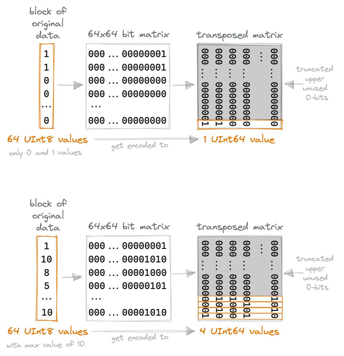
The smaller the maximum value of a block is, the better it compresses. This means T64 is effective when the true column values are very small compared to the range of the data type or if the column is sparsely populated, i.e., only very few values are non-zero. Our columns satisfy one of these conditions, i.e., they are either very sparse or their values are small compared to their UInt16 type. This highlights our point - a codec needs to apply to your data distribution to be effective!

Interestingly, most of the codecs seem to be largely ineffective in the presence of ZSTD, with plain ZSTD (no codec and the Cloud default) offering the 2nd best compression in many cases. ZSTD only consistently benefits when combined with Delta encoding.

A simple query can confirm the most effective codec for each column.

SELECT
    name,
    if(argMin(compression_codec, data_compressed_bytes) != '', argMin(compression_codec, data_compressed_bytes), 'DEFAULT') AS best_codec,
    formatReadableSize(min(data_compressed_bytes)) AS compressed_size
FROM system.columns
WHERE table LIKE 'noaa%'
GROUP BY name

┌─name─────────────┬─best_codec──────────────────┬─compressed_size─┐
│ snowfall         │ CODEC(T64, ZSTD(1))         │ 28.35 MiB       │
│ tempMax          │ CODEC(T64, ZSTD(1))         │ 394.96 MiB      │
│ lat              │ DEFAULT                     │ 3.46 MiB        │
│ tempMin          │ CODEC(T64, ZSTD(1))         │ 382.42 MiB      │
│ date             │ CODEC(DoubleDelta, ZSTD(1)) │ 24.11 MiB       │
│ tempAvg          │ CODEC(T64, ZSTD(1))         │ 101.30 MiB      │
│ lon              │ DEFAULT                     │ 3.47 MiB        │
│ name             │ DEFAULT                     │ 4.20 MiB        │
│ location         │ DEFAULT                     │ 15.00 MiB       │
│ weatherType      │ DEFAULT                     │ 16.30 MiB       │
│ elevation        │ DEFAULT                     │ 1.84 MiB        │
│ station_id       │ DEFAULT                     │ 2.95 MiB        │
│ snowDepth        │ CODEC(ZSTD(1))              │ 41.74 MiB       │
│ precipitation    │ CODEC(T64, ZSTD(1))         │ 408.17 MiB      │
│ averageWindSpeed │ CODEC(T64, ZSTD(1))         │ 9.33 MiB        │
│ maxWindSpeed     │ CODEC(T64, ZSTD(1))         │ 6.14 MiB        │
│ percentDailySun  │ DEFAULT                     │ 1.46 MiB        │
└──────────────────┴─────────────────────────────┴─────────────────┘
✎

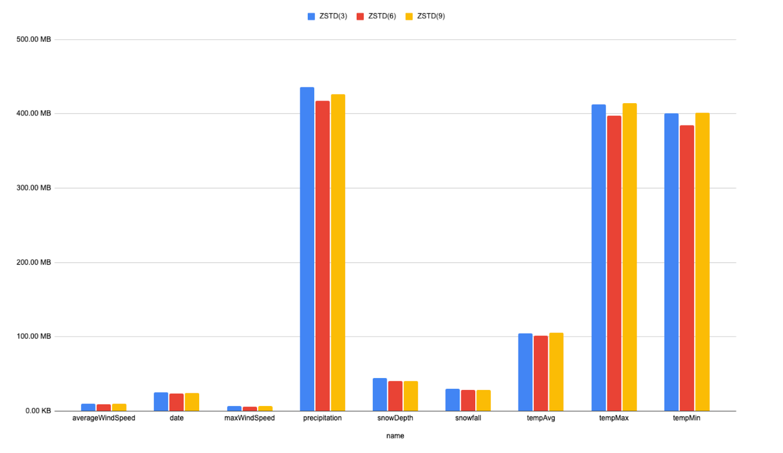
Our current changes achieve considerable storage savings. There are a few ways we can improve this further if storage density is paramount. One option would be to increase the ZSTD compression further. We create a table using the above schema but increase the ZSTD compression level. Below we show the differences for levels 3, 6, and 9.

It's evident that increasing the compression yields little storage reductions in this case, and there would be little to no improvement if we increased it further (max 22). It is unlikely we would pay the decompression penalty incurred at query time for these improvements.

We could further explore here the settings `min_compress_block_size` and `max_compress_block_size`. Increasing these will likely improve compression at the expense of read latency on queries which target a small number of blocks, due to the need to decompress more data. We leave this exercise to the reader.

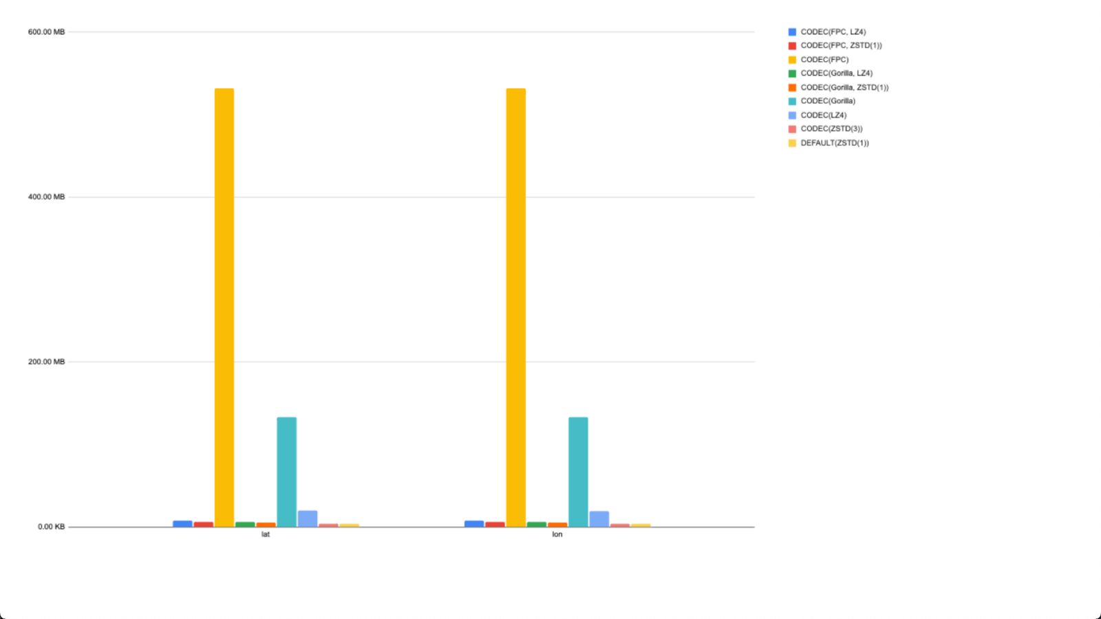
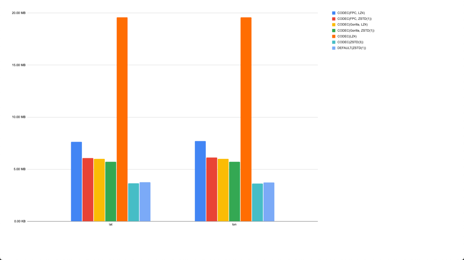
Our final test was to see if we could compress our original location field using the float point codecs Gorilla and FPC. We present the results below, with and without ZSTD and LZ4. Note we still separate our location field into two Float32 columns representing latitude and longitude since we don't need Float64 precision and the waisted bits associated with Point.

Maybe surprisingly, FPC and Gorilla increase our storage requirements. If we remove these columns, we see the plain ZSTD outperforms any codec. There is also no real benefit from increasing the ZSTD compression level to 3.

Our final schema is thus:

CREATE TABLE noaa_codec_optimal
(
   `station_id` LowCardinality(String),
   `date` Date32 CODEC(DoubleDelta, ZSTD(1)),
   `tempAvg` Int16 CODEC(T64, ZSTD(1)),
   `tempMax` Int16 CODEC(T64, ZSTD(1)),
   `tempMin` Int16 CODEC(T64, ZSTD(1)) ,
   `precipitation` UInt16 CODEC(T64, ZSTD(1)) ,
   `snowfall` UInt16 CODEC(T64, ZSTD(1)) ,
   `snowDepth` UInt16 CODEC(ZSTD(1)),
   `percentDailySun` UInt8,
   `averageWindSpeed` UInt16 CODEC(T64, ZSTD(1)),
   `maxWindSpeed` UInt16 CODEC(T64, ZSTD(1)),
   `weatherType` Enum8('Normal' = 0, 'Fog' = 1, 'Heavy Fog' = 2, 'Thunder' = 3, 'Small Hail' = 4, 'Hail' = 5, 'Glaze' = 6, 'Dust/Ash' = 7, 'Smoke/Haze' = 8, 'Blowing/Drifting Snow' = 9, 'Tornado' = 10, 'High Winds' = 11, 'Blowing Spray' = 12, 'Mist' = 13, 'Drizzle' = 14, 'Freezing Drizzle' = 15, 'Rain' = 16, 'Freezing Rain' = 17, 'Snow' = 18, 'Unknown Precipitation' = 19, 'Ground Fog' = 21, 'Freezing Fog' = 22),
   `lat` Float32,
   `lon` Float32,
   `elevation` Int16,
   `name` LowCardinality(String)
)
ENGINE = MergeTree
ORDER BY (station_id, date)

SELECT
    name,
    formatReadableSize(sum(data_compressed_bytes)) AS compressed_size,
    formatReadableSize(sum(data_uncompressed_bytes)) AS uncompressed_size,
    round(sum(data_uncompressed_bytes) / sum(data_compressed_bytes), 2) AS ratio
FROM system.columns
WHERE table = 'noaa_codec_optimal'
GROUP BY name
ORDER BY sum(data_compressed_bytes) DESC

┌─name─────────────┬─compressed_size─┬─uncompressed_size─┬───ratio─┐
│ precipitation    │ 416.51 MiB      │ 2.01 GiB          │    4.93 │
│ tempMax          │ 400.70 MiB      │ 2.01 GiB          │    5.13 │
│ tempMin          │ 388.00 MiB      │ 2.01 GiB          │    5.29 │
│ tempAvg          │ 101.50 MiB      │ 2.01 GiB          │   20.24 │
│ snowDepth        │ 43.48 MiB       │ 2.01 GiB          │   47.24 │
│ snowfall         │ 28.72 MiB       │ 2.01 GiB          │   71.51 │
│ date             │ 24.28 MiB       │ 4.01 GiB          │  169.17 │
│ weatherType      │ 16.90 MiB       │ 1.00 GiB          │   60.76 │
│ averageWindSpeed │ 9.37 MiB        │ 2.01 GiB          │  219.32 │
│ maxWindSpeed     │ 6.17 MiB        │ 2.01 GiB          │  332.67 │
│ name             │ 5.07 MiB        │ 1.98 GiB          │  400.41 │
│ station_id       │ 4.52 MiB        │ 1.97 GiB          │  447.45 │
│ lat              │ 3.64 MiB        │ 4.01 GiB          │ 1128.65 │
│ lon              │ 3.63 MiB        │ 4.01 GiB          │ 1130.98 │
│ elevation        │ 1.93 MiB        │ 2.01 GiB          │ 1066.81 │
│ percentDailySun  │ 1.56 MiB        │ 1.00 GiB          │  658.76 │
└──────────────────┴─────────────────┴───────────────────┴─────────┘
✎

SELECT
    formatReadableSize(sum(data_compressed_bytes)) AS compressed_size,
    formatReadableSize(sum(data_uncompressed_bytes)) AS uncompressed_size,
    round(sum(data_uncompressed_bytes) / sum(data_compressed_bytes), 2) AS ratio
FROM system.columns
WHERE table = 'noaa_codec_optimal'

┌─compressed_size─┬─uncompressed_size─┬─ratio─┐
│ 1.42 GiB        │ 36.05 GiB         │ 25.36 │
└─────────────────┴───────────────────┴───────┘
✎

From our original unoptimized schema, we’ve reduced our uncompressed size from 135GB to around 36GB through type optimizations and reduced our compressed size from 4GB to 1.4GB with codecs.

On the large instance sizes hosting play.clickhouse.com, we wouldn’t expect much performance impact on our query - even the original 4GB compressed size will have fit into local file system caches. The performance for our test query is conversely not negatively affected in this case either with this storage-optimized schema (more queries need testing in reality):

SELECT
    elevation_range,
    uniq(station_id) AS num_stations,
    max(tempMax) / 10 AS max_temp,
    min(tempMin) / 10 AS min_temp,
    sum(precipitation) AS total_precipitation,
    avg(percentDailySun) AS avg_percent_sunshine,
    max(maxWindSpeed) AS max_wind_speed,
    sum(snowfall) AS total_snowfall
FROM noaa_codec_optimal
WHERE (date > '1970-01-01') AND (station_id IN (
    SELECT station_id
    FROM stations
    WHERE country_code = 'US'
))
GROUP BY floor(elevation, -2) AS elevation_range
ORDER BY elevation_range ASC
FORMAT `Null`

0 rows in set. Elapsed: 1.235 sec. Processed 330.20 million rows, 6.48 GB (267.28 million rows/s., 5.25 GB/s.)
 ✎

Choosing which codec and compression algorithm to use ultimately comes down to understanding the characteristics of your data and the properties of the codecs and compression algorithms. While we encourage you to test, we also find the following general guidelines useful to act as a starting point:

• ZSTD all the way - ZSTD with no codec often outperforms other options concerning compression or is at the very least competitive: especially for floating points. This is thus our default compression in ClickHouse Cloud.
• Delta for integer sequences - Delta-based codecs work well whenever you have Monotonic sequences or small deltas in consecutive values. More specifically, the Delta codec works well, provided the derivatives yield small numbers. If not, DoubleDelta is worth trying (this typically adds little if the first-level derivative from Delta is already very small). Sequences where the monotonic increment is uniform, will compress even better - see the dramatic savings on our date field.
• Maybe Gorilla and T64 for unknown patterns - If the data has an unknown pattern, it may be worth trying Gorilla and T64. Gorilla is designed principally for floating point data with small changes in value. It specifically calculates an XOR between the current and previous value and writes it in compact binary form: with the best results when neighboring values are the same. For further information, see Compressing Values in Gorilla: A Fast, Scalable, In-Memory Time Series Database. It can also be used for integers. In our tests, however, plain ZSTD outperforms these codecs even when combined with them.
• T64 for sparse or small ranges - Above, we have shown T64 can be effective on sparse data or when the range in a block is small. Avoid T64 for random numbers.
• Gorilla possibly for floating point and gauge data - Other posts have highlighted Gorilla's effectiveness on floating point data, specifically that which represents gauge readings, i.e., random spikes. This aligns with the algorithmic properties, although we have no fields in our above dataset to verify. Our tests above suggest, at least on Float32s, that ZSTD offers the best compression of Floats.
• Delta improves ZSTD - ZSTD is an effective codec on delta data - conversely, delta encoding can improve ZSTD compression. Compression levels above 3 rarely result in significant gains, but we recommend testing. In the presence of ZSTD, other codecs rarely offer further improvement, as demonstrated by our results above. We have seen reports of LZ4 offering superior compression on DoubleDelta encoded data than ZSTD on artificial datasets, but we have yet to find evidence of this with our real datasets.
• LZ4 over ZSTD if possible - if you get comparable compression between LZ4 and ZSTD, favor the former since it offers faster decompression and needs less CPU. However, ZSTD will outperform LZ4 by a significant margin in most cases. Some of these codecs may work faster in combination with LZ4 while providing similar compression compared to ZSTD without a codec. This will be data specific, however, and requires testing.