While many of the approaches in this blog post remain valid, the content is from 2023. For the latest guidance on migrating data from Postgres to ClickHouse, we recommend exploring newer resources - primarily how ClickPipes, ClickHouse Cloud's managed data ingestion pipeline, now supports ingesting data into ClickHouse from Postgres using CDC.

Introduction #
This post continues our series on the Postgres integrations available in ClickHouse. In our previous post, we explored the Postgres function and table engine, demonstrating how users can move their transactional data to ClickHouse from Postgres for analytical workloads. In this post, we show how Postgres data can also be used in conjunction with the popular ClickHouse dictionary feature to accelerate queries - specifically joins. Finally, we show how the Postgres table engine can be used to push the results of analytical queries back to Postgres from ClickHouse. This "reverse ELT" process can be used for cases where users need to display summarized data in an end-user application but wish to offload the heavy computation of these statistics to ClickHouse.
If you want to dive deeper into these examples and reproduce them, ClickHouse Cloud is a great starting point - spin up a cluster and get $300 of free credit, load the data, let us deal with the infrastructure, and get querying!
We continue to use only a development instance in ClickHouse Cloud for the examples in this post. For our Postgres instance, we also continue with Supabase, which offers a generous free tier sufficient for our examples. We assume the user has loaded the UK house price dataset into ClickHouse as a step from the previous blog post. This dataset can also be loaded without using Postgres using the steps outlined here.
Powering Dictionaries with Postgres #
As we've highlighted in previous blog posts, dictionaries can be used to accelerate ClickHouse queries, especially those involving joins. Consider the following example, where we aim to find the regions for the UK (based on ISO 3166-2) that have experienced the largest price change in the last 20 years. Note that ISO 3166-2 codes are different than postcodes and represent a larger regional area but, more importantly, are useful for visualizing this data in tools such as Superset.
The JOIN requires us to use a list of postcode to regional code mappings, which can be downloaded and loaded into a codes table, as shown below. With over 1 million rows, this takes about a minute to load into our Supabase free tier instance. Let's assume this data is only in Postgres for now, so we will join this in Postgres to answer the query.
Note: our list of postcodes to iso 3166-2 codes were generated from the house price dataset and using a listing of regional codes present in our play.clickhouse.com environment. This dataset, while sufficient for our needs, is therefore not complete or exhaustive, covering only postcodes present in the house price dataset. The query used to generate our file can be found here.
wget https://datasets-documentation.s3.amazonaws.com/uk-house-prices/postgres/uk_postcode_to_iso.sql

psql -c "CREATE TABLE uk_postcode_to_iso
(
        id serial,
    	postcode varchar(8) primary key,
    	iso_code char(6)
);"

psql -c "CREATE INDEX ON uk_postcode_to_iso (iso_code);"
psql < uk_postcode_to_iso.sql

psql -c "select count(*) from uk_postcode_to_iso;"
  count
---------
 1272836
(1 row)

psql -c "\timing" -c "SELECT iso_code, round(avg(((median_2022 - median_2002)/median_2002) * 100)) AS percent_change FROM (
  SELECT postcode1 || ' ' || postcode2 AS postcode, PERCENTILE_CONT(0.5) WITHIN GROUP (ORDER BY price) AS median_2002 FROM uk_price_paid WHERE extract(year from date) = '2002' GROUP BY postcode
) med_2002 INNER JOIN (
  SELECT postcode1 || ' ' || postcode2 AS postcode, PERCENTILE_CONT(0.5) WITHIN GROUP (ORDER BY price) AS median_2022 FROM uk_price_paid WHERE extract(year from date) = '2022' GROUP BY postcode
) med_2022 ON med_2002.postcode=med_2022.postcode INNER JOIN (
	SELECT iso_code, postcode FROM uk_postcode_to_iso
) postcode_to_iso ON med_2022.postcode=postcode_to_iso.postcode GROUP BY iso_code ORDER BY percent_change DESC LIMIT 10;"

Timing is on.

iso_code | percent_change
----------+----------------
 GB-TOF   |        	403
 GB-KEC   |        	380
 GB-MAN   |        	360
 GB-SLF   |        	330
 GB-BGW   |        	321
 GB-HCK   |        	313
 GB-MTY   |        	306
 GB-AGY   |        	302
 GB-RCT   |        	293
 GB-BOL   |        	292
(10 rows)

Time: 48523.927 ms (00:48.524)
The query here is quite complicated and more expensive than the queries in our previous post, which just computed the highest changing postcodes for London. There is no opportunity to exploit the town index, although we can utilize the EXTRACT(year FROM date index as shown by an EXPLAIN.
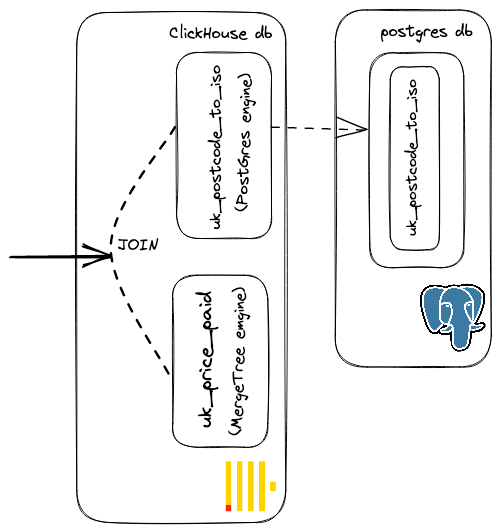
We could also load this iso code data into a ClickHouse table and repeat the join, adjusting the syntax where required. Alternatively, we might be tempted to leave the mapping in Postgres as its subject to reasonably frequent changes. If performing the join in ClickHouse, this produces the following query. Note how we create a uk_postcode_to_iso using the PostgreSQL table engine to simplify the query syntax vs. using the postgres function.

CREATE TABLE uk_postcode_to_iso AS postgresql('db.zcxfcrchxescrtxsnxuc.supabase.co', 'postgres', 'uk_postcode_to_iso', 'postgres', '')

SELECT
	iso_code,
	round(avg(percent_change)) AS avg_percent_change
FROM
(
	SELECT
    	postcode,
    	medianIf(price, toYear(date) = 2002) AS median_2002,
    	medianIf(price, toYear(date) = 2022) AS median_2022,
    	((median_2022 - median_2002) / median_2002) * 100 AS percent_change
	FROM uk_price_paid
	GROUP BY concat(postcode1, ' ', postcode2) AS postcode
	HAVING isNaN(percent_change) = 0
) AS med_by_postcode
INNER JOIN uk_postcode_to_iso ON uk_postcode_to_iso.postcode = med_by_postcode.postcode
GROUP BY iso_code
ORDER BY avg_percent_change DESC
LIMIT 10

┌─iso_code─┬─avg_percent_change─┐
│ GB-TOF   │            	403 │
│ GB-KEC   │            	380 │
│ GB-MAN   │            	360 │
│ GB-SLF   │            	330 │
│ GB-BGW   │            	321 │
│ GB-HCK   │            	313 │
│ GB-MTY   │            	306 │
│ GB-AGY   │            	302 │
│ GB-RCT   │            	293 │
│ GB-BOL   │            	292 │
└──────────┴────────────────────┘

10 rows in set. Elapsed: 4.131 sec. Processed 29.01 million rows, 305.27 MB (7.02 million rows/s., 73.90 MB/s.)
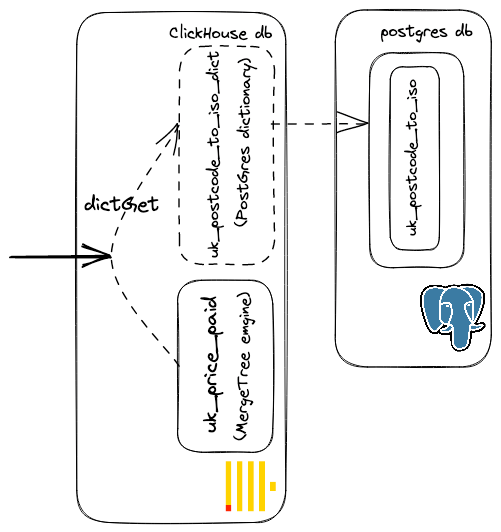
This isn't delivering the performance we would like. Instead of creating a ClickHouse table for the mapping, we can create a PostgreSQL-backed dictionary as shown below:
CREATE DICTIONARY uk_postcode_to_iso_dict
(
`postcode` String,
`iso_code` String
)
PRIMARY KEY postcode
SOURCE(POSTGRESQL(
   port 5432
   host 'db.ebsmckuuiwnvyiniuvdt.supabase.co'
   user 'postgres'
   password ''
   db 'postgres'
   table 'uk_postcode_to_iso'
   invalidate_query 'SELECT max(id) as mid FROM uk_postcode_to_iso'
))
LIFETIME(300)
LAYOUT(complex_key_hashed())

//force loading of dictionary
SELECT dictGet('uk_postcode_to_iso_dict', 'iso_code', 'BA5 1PD')

┌─dictGet('uk_postcode_to_iso_dict', 'iso_code', 'BA5 1PD')─┐
│ GB-SOM                                                	│
└───────────────────────────────────────────────────────────┘

1 row in set. Elapsed: 0.885 sec.
This dictionary will periodically update based on the LIFETIME clause, automatically syncing any changes. In this case, we also define an invalidate_query clause which controls when the dataset needs to be reloaded from the source by returning a single value. If this changes, the dictionary is reloaded - in this case, when the max id changes. In a production scenario, we would probably want a query capable of detecting updates via a modified time field.

Using this dictionary, we can now modify our query and exploit the fact that this table is held locally in memory for fast lookups. Note how we can also avoid the join:
SELECT
	iso_code,
	round(avg(percent_change)) AS avg_percent_change
FROM
(
	SELECT
    	dictGet('uk_postcode_to_iso_dict', 'iso_code', postcode) AS iso_code,
    	medianIf(price, toYear(date) = 2002) AS median_2002,
    	medianIf(price, toYear(date) = 2022) AS median_2022,
    	((median_2022 - median_2002) / median_2002) * 100 AS percent_change
	FROM uk_price_paid
	GROUP BY concat(postcode1, ' ', postcode2) AS postcode
	HAVING isNaN(percent_change) = 0
)
GROUP BY iso_code
ORDER BY avg_percent_change DESC
LIMIT 10

┌─iso_code─┬─avg_percent_change─┐
│ GB-TOF   │            	403 │
│ GB-KEC   │            	380 │
│ GB-MAN   │            	360 │
│ GB-SLF   │            	330 │
│ GB-BGW   │            	321 │
│ GB-HCK   │            	313 │
│ GB-MTY   │            	306 │
│ GB-AGY   │            	302 │
│ GB-RCT   │            	293 │
│ GB-BOL   │            	292 │
└──────────┴────────────────────┘

10 rows in set. Elapsed: 0.444 sec. Processed 27.73 million rows, 319.84 MB (62.47 million rows/s., 720.45 MB/s.)
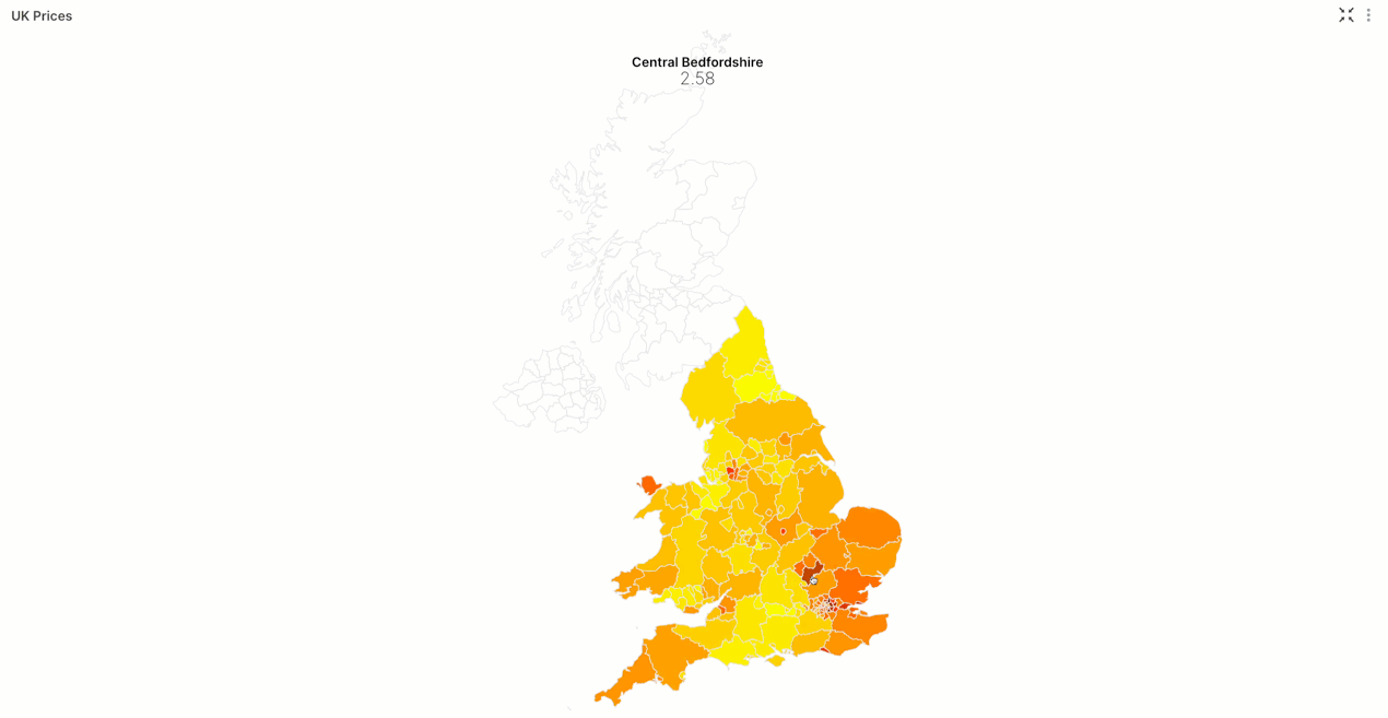
That's better. For those interested, this data is plottable in tools such as Superset, which can interpret these iso-codes - see our previous blog post on Superset for a similar example.

Pushing Results to Postgres #
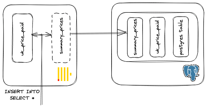
Up to now, we’ve demonstrated the value of moving data to ClickHouse from Postgres for analytical workloads. If we consider this as an ETL process, it is likely that at some point, we will want to reverse this workflow and load the results of our analysis back into Postgres. We can achieve this using the same table engine we highlighted earlier in this series.

Suppose we wanted to push aggregate statistics back to Postgres for the sales during each month, summarized by postcode, type, whether the house is new, and if it's a freehold or leasehold. Our hypothetical site will display these statistics on every page of a listing to help its users understand the historical market conditions in an area. Additionally, they would like to be able to display these statistics over time. To lower the load* on their production Postgres instance, they offload this computation to ClickHouse and periodically push these results back to a summary table.
In reality, this isn't a particularly heavy query and could probably be scheduled in Postgres.
Below we create a ClickHouse database backed by Postgres before creating a table and inserting the results of our analytical query.
CREATE TABLE summary_prices(
postcode1 varchar(8),
            	type varchar(13),
            	is_new SMALLINT,
            	duration varchar(9),
            	sold integer,
            	month Date,
            	avg_price integer,
            	quantile_prices integer[]);

// create Postgres engine table in ClickHouse
CREATE TABLE summary_prices AS postgresql('db.zcxfcrchxescrtxsnxuc.supabase.co', 'postgres', 'summary_prices', 'postgres', '')

//check connectivity
SELECT count()
FROM summary_prices

┌─count()─┐
│       0 │
└─────────┘

1 row in set. Elapsed: 0.337 sec.

// insert the result of our query to Postgres
INSERT INTO summary_prices SELECT
	postcode1,
	type,
	is_new,
	duration,
	count() AS sold,
	month,
	avg(price) AS avg_price,
	quantilesExactExclusive(0.25, 0.5, 0.75, 0.9, 0.95, 0.99)(price) AS quantile_prices
FROM uk_price_paid
WHERE postcode1 != ''
GROUP BY
	toStartOfMonth(date) AS month,
	postcode1,
	type,
	is_new,
	duration
ORDER BY
	postcode1 ASC,
	type ASC,
	is_new ASC,
	duration ASC,
	month ASC

0 rows in set. Elapsed: 25.714 sec. Processed 27.69 million rows, 276.98 MB (775.43 thousand rows/s., 7.76 MB/s.)
Our site now has a simple query to run to fetch the historical price statistics for an area and house of the same type.
postgres=> SELECT postcode1, month, avg_price, quantile_prices FROM summary_prices WHERE postcode1='BA5' AND type='detached' AND is_new=0 and duration='freehold' LIMIT 10;
 postcode1 |   month    | avg_price |              quantile_prices
-----------+------------+-----------+--------------------------------------------
 BA5       | 1995-01-01 |    108000 | {64000,100000,160000,160000,160000,160000}
 BA5       | 1995-02-01 |     95142 | {86500,100000,115000,130000,130000,130000}
 BA5       | 1995-03-01 |    138991 | {89487,95500,174750,354000,354000,354000}
 BA5       | 1995-04-01 |     91400 | {63750,69500,130000,165000,165000,165000}
 BA5       | 1995-05-01 |    110625 | {83500,94500,149750,170000,170000,170000}
 BA5       | 1995-06-01 |    124583 | {79375,118500,173750,185000,185000,185000}
 BA5       | 1995-07-01 |    126375 | {88250,95500,185375,272500,272500,272500}
 BA5       | 1995-08-01 |    104416 | {67500,95000,129750,200000,200000,200000}
 BA5       | 1995-09-01 |    103000 | {70000,97000,143500,146000,146000,146000}
 BA5       | 1995-10-01 |     90800 | {58375,72250,111250,213700,223000,223000}
(10 rows)
Conclusion #
In this series of posts, we have shown how ClickHouse and Postgres are complementary, demonstrating with examples of how data can be moved effortlessly between the two databases using the native ClickHouse functions and table engines. In this specific post, we have covered a Postgres-backed dictionary and how it can be used to accelerate joins for queries involving a frequently changing dataset. Finally, we have performed a “reverse ETL” operation, pushing the results of an analytical query back to Postgres for consumption from a possible user-facing application.


