Resmo is a tool that gathers configuration data from Cloud and SaaS tools using APIs, and users can explore this data using SQL to ask any question they want. Resmo comes with thousands of pre-built SQL-based rules and questions and also provides visual exploration capabilities of the collected data through filters, free text search or graph. Customers can create their own rules or use automation to receive notifications via various channels when there are changes to the data or rule status.
Collecting configuration data from 1000s of APIs results in a large number of network calls, especially when considering RESTful APIs that require multiple requests to retrieve complete data. Despite the API services working most of the time, occasional issues such as network failures or server outages can occur for many reasons, per service or per customer. Therefore, it's important to have a rock-solid observability to monitor the system's health, detect anomalies, and identify the root cause of failures quickly.
However, the traditional approach of logs can be too verbose and hard to query. On the other hand, aggregated metrics may not provide enough context, making them less useful for detecting and diagnosing specific issues. Therefore, at Resmo we utilize tracing, which provides a better view of the flow of requests and their associated responses.This approach allows us to efficiently store and query traces, a challenge common to time-series database workloads, which can quickly add up, considering the thousands of API calls per customer every 10 minutes. Today, there are more than 300 million spans generated by Resmo data collection per day and it is increasing rapidly with the customer size.
The usual approach to excessive volume of spans would be sampling. However, this can cause blind spots, making it difficult to identify issues on non-happy paths of execution that happen rarely. To avoid this, at Resmo, we’ve chosen to use full tracing (no sampling) with OpenTelemetry but we still need to be cost effective. Many traditional observability vendors charge by the number of ingested events or per-user, which can become costly without aggressive sampling. This restrictive model is a primary reason engineering teams seek out cost-effective alternatives to platforms like New Relic. Furthermore, only a handful of these vendors allow you to run custom SQL queries on that data.
At first, we wanted to utilize S3 and Athena. We’ve forked the OpenTelemetry collector to produce Parquet files directly to S3, adding very common span attributes (i.e tenant and user IDs) as additional columns for efficient querying. But, even though Athena can query vast amounts of data, it has a fixed startup delay of 2-3 seconds. This can be annoying for the most simplistic queries, i.e we lookup traces by just IDs, or simple slice-and-dice aggregations. Additionally, for efficiency the Parquet files were generated every 60 seconds. Athena performance degrades by the number of files generated and in the end we’d still get delayed data. Realizing Athena may not be the best way to move forward, we’ve decided to try ClickHouse. There was already an exporter available in the OpenTelemetry contrib repository. Although it’s in alpha status, since our implementation 3 months ago we have not faced any problems.
Storage and compression
We host our own ClickHouse instance, as the automated instrumentation by OpenTelemetry Java Agent can also put sensitive values in the spans. It’s also a cost effective way to approach the problem. With a single c7g.xlarge node, with 4 CPUs based on Graviton3, and 400 GB of provisioned EBS disk, we can store more than 4 billion spans. This consumes 275 GiB on disk, which uncompressed is 3.40 TiB - a %92 compression percentage, pretty impressive! If a query is scanning lots of data, the computation is usually IO bound and cannot fully utilize all of the CPUs. If we have used instances with local disks and S3 as tiered storage, we might have better performance and longer retention. However, our current setup is mostly sufficient unless we scan billions of rows.
Customization and lessons learned
To improve the performance of common queries, we add materialized columns for those frequently used in queries, monitors, and dashboards: such as tenant and user IDs, and some span-specific fields like URLs. These new columns are LowCardinality strings and significantly improved query performance without affecting storage or the compression rate. When adding new materialized columns, always check their status from the system.mutations table to avoid issues. Although the ALTER TABLE command may finish quickly, the actual materialization process requires reading all data and executing expressions.
To implement distributed tracing, we’ve used the out of the box configuration of Opentelemetry Collector with ClickHouse and Java agent. Although automatic Java instrumentation works in most cases, we have also added some manual instrumentation in the form of context specific tags to our spans e.g. tenant IDs, user IDs, domain specific tags, or custom measurements related to our business functions.
Instrumentation, queries and insights
Traditional distributed tracing services often focus on basic monitoring using durations, as well as simple group by aggregations for service discovery, finding bottlenecks and critical paths. While all useful, the ability to write SQL gives us unprecedented flexibility. As lovers of SQL at Resmo, we were keen to expose this flexibility to our customers so they can easily ask arbitrary questions.
Another useful feature of ClickHouse is that it can be easily connected to Postgres, allowing us to use it in our observability queries. For example, we can join the user and tenant IDs in our spans to the actual account names and account status in the Postgres database. In our future roadmap, we want to try the MateralizedPostgreSQL engine for improved performance. We also plan to make use of dictionaries to simplify some of the queries.
For visualizing data we use Grafana. The ClickHouse plugin, which has a nice query builder and also provides useful macros for time series filtering, allows us to visualize the spans over time. We also make use of IntelliJ IDEA & DataGrip to connect to ClickHouse and write our queries. The progress bar on the CLI is what makes it so great, giving us a clear indication of how well the query is running. It was surprising to see how fast even complex queries progressed at first, but now I'm used to it and can't imagine using anything else.

While there are open source options like SigNoz and Uptrace that use ClickHouse as their foundation, we opted to work with ClickHouse directly to deepen our understanding of it, particularly as we began transitioning some of our high-volume data to the platform. We have included some of our more common queries below to benefit others.
Average and percentile duration of spans
This is the most obvious and easy one, but also one of the most used. Because often we want to search for outliers, and drill down from there to specific time frame, function, tenant or customer. Remember to always include a Timestamp filter, otherwise the query will end up scanning all the data. To make quick exploration easier, we created views as traces5m, traces1h, traces4h and traces1d to avoid filtering by timestamp all the time. We also created a parameterized view, that can filter on any arbitrary hours to simplify ad-hoc queries:
CREATE VIEW traces AS
SELECT *
FROM otel_traces
WHERE Timestamp > (NOW() - toIntervalHour({hr:Int}))
SELECT COUNT(*) FROM traces(hr=5)Queries which do scan all of the data also complete rather quickly, compared to what we’d normally expect, and are mostly limited by the disk bandwidth. Currently we use EBS, but we also plan to experiment with S3 backed storage with local disks, various CPU types and memory settings.
SELECT
SpanName,
COUNT(*),
avg(DurationMs),
quantile(0.9)(DurationMs) AS p90,
quantile(0.95)(DurationMs) AS p95,
quantile(0.99)(DurationMs) AS p99
FROM otel.otel_traces
WHERE Timestamp > NOW() - toIntervalHour(24)
GROUP BY 1
ORDER BY p99 DESC
LIMIT 10Combining data in Aurora PostgreSQL with ClickHouse
At Resmo, we primarily utilize Aurora Postgres to store our application data. Spans are generated using ClickHouse through automatic instrumentation. We create a new root span with account_id and user_id for every incoming HTTP request or asynchronous message that is processed from SQS.
Rate Limiting functionality in our product is manually instrumented with various keys. However, to avoid errors during testing, E2E tests are exempted from this instrumentation, and a shared secret is passed through an HTTP header for quick implementation. To monitor usage, the spans where the rate limit check happens are identified with another attribute.
Since the inner rate limiting span lacks an account ID attribute, it's necessary to leverage SQL joins to identify this within the inner spans by referencing the root span. The span is then joined with the Postgres table containing account names, eliminating the need to duplicate account IDs to every span and lookup account names in manual instrumentation. Although it might look complex, it’s a very good example of why we love SQL.
SELECT a.name AS accountName,
count(1)
FROM otel.otel_traces t
JOIN default.accounts a ON t.account_id = a.id
WHERE Timestamp > NOW() - interval 48 HOUR
AND ParentSpanId = ''
AND TraceId IN
(SELECT DISTINCT TraceId
FROM otel.otel_traces
WHERE Timestamp > NOW() - interval 48 HOUR
AND SpanName = 'RateLimiterService.checkLimit'
AND SpanAttributes['rate_limiter.bypassed'] = 'true')
AND account_id != ''
GROUP BY 1Get insights on SpanAttributes
Although automatic instrumentation provides a lot of valuable information, it can be challenging to navigate through it all. Map functions can assist in analyzing SpanAttributes by counting the number of keys and assessing the uniqueness of their values. This approach can help you explore the data in greater depth. However, it's essential to note that the query reads all of the SpanAttributes map, which constitutes the majority of the trace data. As a result, querying the data for an entire day can take a significant amount of time - approximately 90 seconds in our case. Nevertheless, given the vast amount of data this query reads, the performance is still excellent. Please be aware that some of the output is removed for privacy reasons.
WITH x AS
(
SELECT untuple(arrayJoin(SpanAttributes)) AS x
FROM traces1d
)
SELECT
`x.1` AS key,
uniqExact(`x.2`) AS unqiues,
count(1) AS total
FROM x
GROUP BY 1
ORDER BY 2 DESC
LIMIT 50
┌─key──────────────────────────────────┬─unqiues─┬─────total─┐
│ poller.sqs.message_id │ 2903676 │ 2907976 │
│ thread.name │ 2811101 │ 312486284 │
│ http.url │ 1737533 │ 31551967 │
│ requestId │ 62068 │ 62078 │
│ net.peer.name │ 1352 │ 147641850 │
│ aws.bucket.name │ 1179 │ 757770 │
│ http_request.referer │ 356 │ 6904 │
│ rpc.method │ 315 │ 28193140 │
│ db.sql.table │ 53 │ 2822582 │
└──────────────────────────────────────┴─────────┴───────────┘
50 rows in set. Elapsed: 93.042 sec. Processed 314.64 million rows, 141.35 GB (3.38 million rows/s., 1.52 GB/s.)It's apparent that the most frequent keys are thread names, which are created automatically. However, our Aurora databases are consistently queried by SQL queries, resulting in only 53 tables being accessed out of the 2.8 million database calls. Fields like message or request IDs tend to be mostly unique.
Analyzing the distribution of your data and keys can enable you to create materialized fields and offer additional opportunities to explore the data in greater depth.
Tracing hygiene and debugging
Although automatic instrumentation can be extremely beneficial, it may generate an overwhelming number of spans, making it difficult to navigate through them. Furthermore, if you add your own spans and attributes, your dataset can become congested, making debugging more challenging. To determine whether you are collecting valuable data, you can again simply use SQL!
One option is to evaluate the number of spans per trace. This was particularly important for us, as some of our traces contain many network calls. Each of the network calls are represented as a span. Ideally, a single trace should consist of unit work as much as possible for reliability, and not contain thousands of network calls. The SQL query below calculates the number of spans per trace and creates a histogram. To visualize the output in the CLI, we can use the built-in bar function. Additionally, the log function is utilized to create a more comprehensible graph.
WITH histogram(10)(total) AS hist
SELECT
round(arrayJoin(hist).1) AS lower,
round(arrayJoin(hist).2) AS upper,
arrayJoin(hist).3 AS cnt,
bar(log(cnt), 0, 32) AS bar
FROM
(
SELECT
TraceId,
COUNT(*) AS total
FROM traces1d
GROUP BY 1
ORDER BY 2 ASC
)
Query id: 74363105-dc0b-4d07-a591-f4096d7302cf
┌─lower─┬─upper─┬────────cnt─┬─bar─────────────────────────────────────┐
│ 1 │ 144 │ 6232778.75 │ ███████████████████████████████████████ │
│ 144 │ 453 │ 1263445 │ ███████████████████████████████████ │
│ 453 │ 813 │ 206123.75 │ ██████████████████████████████▌ │
│ 813 │ 1300 │ 28555 │ █████████████████████████▋ │
│ 1300 │ 1844 │ 923.75 │ █████████████████ │
│ 1844 │ 2324 │ 166.125 │ ████████████▊ │
│ 2324 │ 2898 │ 94.5 │ ███████████▎ │
│ 2898 │ 3958 │ 24.625 │ ████████ │
│ 3958 │ 5056 │ 65 │ ██████████▍ │
│ 5056 │ 5537 │ 12.5 │ ██████▎ │
└───────┴───────┴────────────┴─────────────────────────────────────────┘
10 rows in set. Elapsed: 7.958 sec. Processed 314.47 million rows, 15.41 GB (39.52 million rows/s., 1.94 GB/s.)Over the last 24 hours, there were over 1000 traces that contained more than 1300 spans each. This could potentially pose a problem. However, at Resmo, we make numerous pagination calls and must execute additional calls for each of them in some integrations, so this level of span volume is anticipated.
Searching Java exception messages
With our backends using Kotlin, automatic instrumentation places any exception messages in the expected format in the Events field of a Span. We can search these using ClickHouse string functions. Normally, we create alerts for important exceptions and route them to OpsGenie. However data collections are prone to intermittent errors and we thus aggregate them. The following query searches for tokens in the exception messages using the hasToken function. You can also use the multiSearchAny function, but it looks anywhere in the string and can yield a large number of results.
The most impressive part is that this data is not indexed at all (e.g. using inverted indices) and searching for a days worth of data can still be done in under 5 seconds.
SELECT
SpanName,
arrayJoin(Events.Attributes)['exception.message'] AS message,
count(1)
FROM traces1d
WHERE (message != '') AND hasToken(lower(message), 'exceeded')
GROUP BY
1,
2
ORDER BY 3 DESC
LIMIT 20
10 rows in set. Elapsed: 4.583 sec. Processed 314.64 million rows, 20.67 GB (68.66 million rows/s., 4.51 GB/s.)Show the compression stats for Materialized Columns
Adding materialized columns speeds-up queries, but they also come at additional storage cost. Before creating a materialized column for every attribute in the SpanAttributes, you should determine whether the performance would justify the additional storage cost. While SpanAttributes and ResourceAttributes take up the most space, currently they have an impressive 14-15x compression ratio. The size of our materialized columns can also be seen in the results, with http.url being a notable example. Despite a 59 GB uncompressed size, it compresses to 3.30 GB with an 18x rate - as most URLs tend to be similar. Lower cardinality columns like integration_id have an even impressive 80x compression rate.
SELECT
name,
name,
formatReadableSize(sum(data_compressed_bytes)) AS compressed_size,
formatReadableSize(sum(data_uncompressed_bytes)) AS uncompressed_size,
round(sum(data_uncompressed_bytes) / sum(data_compressed_bytes), 2) AS ratio
FROM system.columns
WHERE table = 'otel_traces' AND default_expression != ''
GROUP BY name
ORDER BY sum(data_compressed_bytes) DESC
┌─name──────────────┬─compressed_size─┬─uncompressed_size─┬──ratio─┐
│ DurationMs │ 14.64 GiB │ 14.72 GiB │ 1.01 │
│ http.url │ 2.57 GiB │ 46.00 GiB │ 17.92 │
│ topDomain │ 163.23 MiB │ 28.19 GiB │ 176.84 │
│ account_id │ 96.93 MiB │ 6.73 GiB │ 71.15 │
│ net.peer.name │ 79.11 MiB │ 7.36 GiB │ 95.2 │
│ db_statement │ 67.39 MiB │ 4.64 GiB │ 70.51 │
│ integration_id │ 51.50 MiB │ 7.17 GiB │ 142.61 │
│ account_domain │ 46.33 MiB │ 4.55 GiB │ 100.48 │
│ datasave_resource │ 41.01 MiB │ 4.09 GiB │ 102.01 │
│ user_id │ 27.86 MiB │ 3.74 GiB │ 137.29 │
│ integration_type │ 16.89 MiB │ 3.70 GiB │ 224.5 │
│ rpc.service │ 12.29 MiB │ 3.70 GiB │ 308.63 │
│ rpc.system │ 12.21 MiB │ 3.70 GiB │ 310.65 │
│ account_name │ 12.15 MiB │ 3.70 GiB │ 312.13 │
│ hostname │ 12.13 MiB │ 3.70 GiB │ 312.76 │
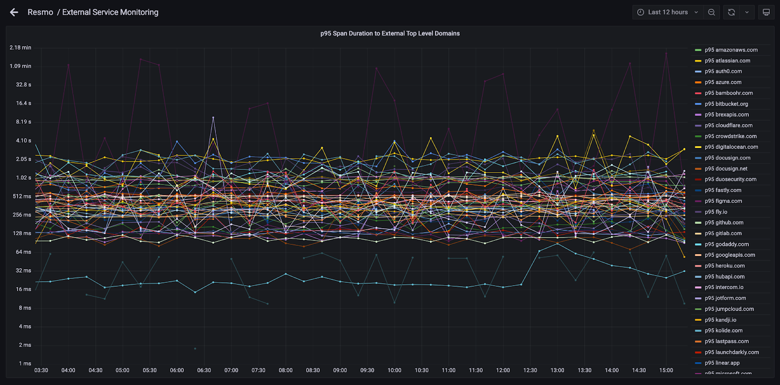
└───────────────────┴─────────────────┴───────────────────┴────────┘One particularly interesting column is topDomain, which extracts domain names from automatic instrumentation values like net.peer.domain to pinpoint networking issues. Although not a perfect solution and this seems very hacky, it provides a good enough summary that we can later drill down on. We use the following function to split the reversed domain name by dot, getting the 1st and 2nd, and reverse it again.
`topDomain` String DEFAULT reverse(concat(splitByChar('.', reverse(net.peer.name))[1], '.', splitByChar('.', reverse(net.peer.name))[2]))By calculating and materializing this expression at the time of ingestion, we can easily create the following Grafana dashboard to visually identify external service performance:
Summary
Within 3 months we have deployed a production tracing solution using ClickHouse with minimal issues. With high compression, full SQL support and excellent query times, even on moderate hardware, we recommend ClickHouse as a store for your tracing data.
Visit: www.resmo.com
To read more about storing trace data in ClickHouse, see our recent blog on using OpenTelemetry.


