ClickHouse Release 24.8 LTS

Another month goes by, which means it’s time for another release!

ClickHouse version 24.8 contains 19 new features 🎁 18 performance optimisations 🛷 65 bug fixes 🐛

This release is an LTS (Long Term Support) one, which means it will be supported for 12 months after release. To learn more about Stable and LTS releases, see the documentation.

In this release, we’ve got the newly revamped JSON type, a table engine for time-series data, exactly-once processing of Kafka messages, and of course, join improvements!

As always, we send a special welcome to all the new contributors in 24.9! ClickHouse's popularity is, in large part, due to the efforts of the community that contributes. Seeing that community grow is always humbling.

Below are the names of the new contributors:

Graham Campbell, Halersson Paris, Jacob Reckhard, Lennard Eijsackers, Miсhael Stetsyuk, Peter Nguyen, Ruihang Xia, Samuele Guerrini, Sasha Sheikin, Vladimir Varankin, Zhukova, Maria, heguangnan, khodyrevyurii, sakulali, shiyer7474, xc0derx, zoomxi

Hint: if you’re curious how we generate this list… here.

You can also view the slides from the presentation.

This release sees the experimental release of the new JSON data type. This has been in the works for a while, and in previous release posts, we’ve talked about a couple of types that it relies on—Variant and Dynamic.

The JSON data type is used to store semi-structured data where the structure of each row might not be the same as that of other rows or where we don’t want to break it out into individual columns.

We will try out this functionality using a football/soccer dataset provided by StatsBomb. The dataset contains matches, lineups, and events.

The most interesting data for our purposes are events. These events could be passes, clearances, blocks, or other things that can happen in a match. Events of the same type have the same structure, but different event types have different fields.

If you want to follow along, you can download the dataset by running the following command:

wget https://github.com/statsbomb/open-data/archive/refs/heads/master.zip

Next, let’s have a quick look at the data we’ll be working with. We’ll read the data in JsonAsObject format so that ClickHouse doesn’t try to infer the types of each property in the JSON.

SELECT
    replaceRegexpAll(splitByRegexp('/', _file)[-1], '.json', '') AS matchId,
    json
FROM file('master.zip :: **/data/events/*.json', JSONAsObject)
LIMIT 1
FORMAT Vertical

Row 1:
──────
matchId: 15946
json:    {"duration":0,"id":"9f6e2ecf-6685-45df-a62e-c2db3090f6c1","index":"1","minute":"0","period":"1","play_pattern":{"id":"1","name":"Regular Play"},"possession":"1","possession_team":{"id":"217","name":"Barcelona"},"second":"0","tactics":{"formation":"442","lineup":[{"jersey_number":"1","player":{"id":"20055","name":"Marc-André ter Stegen"},"position":{"id":"1","name":"Goalkeeper"}},{"jersey_number":"2","player":{"id":"6374","name":"Nélson Cabral Semedo"},"position":{"id":"2","name":"Right Back"}},{"jersey_number":"3","player":{"id":"5213","name":"Gerard Piqué Bernabéu"},"position":{"id":"3","name":"Right Center Back"}},{"jersey_number":"23","player":{"id":"5492","name":"Samuel Yves Umtiti"},"position":{"id":"5","name":"Left Center Back"}},{"jersey_number":"18","player":{"id":"5211","name":"Jordi Alba Ramos"},"position":{"id":"6","name":"Left Back"}},{"jersey_number":"5","player":{"id":"5203","name":"Sergio Busquets i Burgos"},"position":{"id":"9","name":"Right Defensive Midfield"}},{"jersey_number":"4","player":{"id":"5470","name":"Ivan Rakitić"},"position":{"id":"11","name":"Left Defensive Midfield"}},{"jersey_number":"20","player":{"id":"6379","name":"Sergi Roberto Carnicer"},"position":{"id":"12","name":"Right Midfield"}},{"jersey_number":"11","player":{"id":"5477","name":"Ousmane Dembélé"},"position":{"id":"16","name":"Left Midfield"}},{"jersey_number":"9","player":{"id":"5246","name":"Luis Alberto Suárez Díaz"},"position":{"id":"22","name":"Right Center Forward"}},{"jersey_number":"10","player":{"id":"5503","name":"Lionel Andrés Messi Cuccittini"},"position":{"id":"24","name":"Left Center Forward"}}]},"team":{"id":"217","name":"Barcelona"},"timestamp":"00:00:00.000","type":{"id":"35","name":"Starting XI"}}

This row represents a Starting XI event, but several hundred other event types exist. Let’s see how to load this data into ClickHouse.

To use the JSON data type, we’ll need to enable the following:

SET allow_experimental_json_type=1;

Next, we’re going to create an events table. We’ll have a json column that will store the JSON for each event and a matchId column to store the match id, which we’ll extract from the file name.

When creating a ClickHouse table, we must define a sorting key that will impact how the data is sorted on disk. Our key will be the team ID, accessible under possession_team.id.

We can’t make a nested field the sorting key for a table at the moment, but this feature is planned for future versions. For now, we’ll create a column of type MATERIALIZED that pulls the value from the JSON column. We’ll use the materialized column as the sorting key. The table creation query is shown below:

CREATE TABLE events
(
    matchId String,
    json JSON,
    possession_team_id String MATERIALIZED getSubcolumn(json, 'possession_team.id')
)
ENGINE = MergeTree
ORDER BY possession_team_id;

We can then copy our previous SELECT query and prefix it with INSERT INTO events to load the data:

INSERT INTO events 
SELECT
    replaceRegexpAll(splitByRegexp('/', _file)[-1], '.json', '') AS matchId,
    json
FROM file('master.zip :: **/data/events/*.json', JSONAsObject)

0 rows in set. Elapsed: 72.967 sec. Processed 12.08 million rows, 10.39 GB (165.60 thousand rows/s., 142.42 MB/s.)
Peak memory usage: 3.52 GiB.

It takes a little over one minute from the output to load 12 million events. We can then write a query that uses JSON dot syntax to find the most popular types of events:

SELECT
    json.type.name,
    count() AS count
FROM events
GROUP BY ALL
ORDER BY count DESC
LIMIT 10

┌─json.type.name─┬───count─┐
│ Pass           │ 3358652 │
│ Ball Receipt*  │ 3142664 │
│ Carry          │ 2609610 │
│ Pressure       │ 1102075 │
│ Ball Recovery  │  363161 │
│ Duel           │  255791 │
│ Clearance      │  157713 │
│ Block          │  130858 │
│ Dribble        │  121105 │
│ Goal Keeper    │  105390 │
└────────────────┴─────────┘

The dot syntax is useful when we want to read literal values, but it doesn’t work if we read subobjects. For example, the following query counts the most popular possesion_team:

SELECT
    json.possession_team AS team,
    count()
FROM events
GROUP BY team
ORDER BY count() DESC
LIMIT 10

┌─team─┬──count()─┐
│ ᴺᵁᴸᴸ │ 12083338 │
└──────┴──────────┘

Hmmm, all nulls!

The dot syntax doesn’t read nested objects for performance reasons. The data is stored so that reading literal values by paths is very efficient, but reading all subobjects by path requires much more data and can sometimes be slower.

When we want to return an object, we need to use .^ instead. This special syntax can only be used to read nested objects from fields with the JSON data type:

SELECT
    json.^possession_team AS team,
    count()
FROM events
GROUP BY team
ORDER BY count() DESC
LIMIT 10

┌─team──────────────────────────────────────┬─count()─┐
│ {"id":"217","name":"Barcelona"}           │ 1326515 │
│ {"id":"131","name":"Paris Saint-Germain"} │  239930 │
│ {"id":"1","name":"Arsenal"}               │  154789 │
│ {"id":"904","name":"Bayer Leverkusen"}    │  147473 │
│ {"id":"220","name":"Real Madrid"}         │  135421 │
│ {"id":"968","name":"Arsenal WFC"}         │  131637 │
│ {"id":"746","name":"Manchester City WFC"} │  131017 │
│ {"id":"971","name":"Chelsea FCW"}         │  115761 │
│ {"id":"212","name":"Atlético Madrid"}     │  110893 │
│ {"id":"169","name":"Bayern Munich"}       │  104804 │
└───────────────────────────────────────────┴─────────┘

If you’re reading down through multiple nested subobjects and want to return a subobject, you only need to use the .^ syntax for the first object in the path. For example:

select json.^pass.body_part AS x, toTypeName(x)
FROM events 
LIMIT 1;

┌─x───────────────────────────────┬─toTypeName(x)─┐
│ {"id":"40","name":"Right Foot"} │ JSON          │
└─────────────────────────────────┴───────────────┘

This syntax is only intended for returning objects. If you try to use it to return a literal value, you’ll get back an empty JSON object:

SELECT
    json.^possession_team.name AS team, toTypeName(team),
    count()
FROM events
GROUP BY team
ORDER BY count() DESC
LIMIT 10;

┌─team─┬─toTypeName(team)─┬──count()─┐
│ {}   │ JSON             │ 12083338 │
└──────┴──────────────────┴──────────┘

We plan to add a new operator, .$, which will return both literals and subobjects as a single subcolumn.

When we return literal values, their type will be Dynamic. We can use the dynamicType function to determine the underlying type for each value:

SELECT
    json.possession_team.name AS team,
    dynamicType(team) AS teamType,
    json.duration AS duration,
    dynamicType(duration) AS durationType
FROM events
LIMIT 1

┌─team────┬─teamType─┬─duration─┬─durationType─┐
│ Arsenal │ String   │ 0.657763 │ Float64      │
└─────────┴──────────┴──────────┴──────────────┘

We can also use suffixes of.:<Type> to assume a data type and ::<Type> to cast to a data type.

SELECT
    json.possession_team.name AS team,
    toTypeName(team),
    json.possession_team.name.:String AS teamAssume,
    toTypeName(teamAssume) AS assumeType,
    json.possession_team.name::String AS teamCast,
    toTypeName(teamCast) AS castType
FROM events
LIMIT 1;

┌─team────┬─toTypeName(team)─┬─teamAssume─┬─assumeType───────┬─teamCast─┬─castType─┐
│ Arsenal │ Dynamic          │ Arsenal    │ Nullable(String) │ Arsenal  │ String   │
└─────────┴──────────────────┴────────────┴──────────────────┴──────────┴──────────┘

One final thing to note is that columns with the JSON data type can be configured further. For example, if we want to exclude some parts of the JSON objects being stored, we can skip particular paths during JSON pathing using SKIP and SKIP REGEXP.

For example, the following table creation statement skips the pass.body.part path and any path that starts with the letter t:

CREATE TABLE events2
(
    matchId String,
    json JSON(
      SKIP pass.body_part, 
      SKIP REGEXP 't.*'
    ),
    possession_team_id String MATERIALIZED getSubcolumn(json, 'possession_team.id')
)
ENGINE = MergeTree
ORDER BY possession_team_id;

When ingesting data into a table with a JSON column with extra settings, ClickHouse won’t automatically cast the incoming data to the right type, but that will be fixed in a future version. For now, we need to define the JSON column type in our import query explicitly:

INSERT INTO events2
SELECT
    replaceRegexpAll(splitByRegexp('/', _file)[-1], '.json', '') AS matchId,
    json
FROM file(
  'master.zip :: **/data/events/*.json',
  JSONAsObject,
  '`json` JSON(SKIP `pass.body_part`, SKIP REGEXP \'t.*\')'
);

0 rows in set. Elapsed: 75.122 sec. Processed 12.08 million rows, 10.39 GB (160.85 thousand rows/s., 138.33 MB/s.)
Peak memory usage: 3.52 GiB.

If we query events2, we’ll see that those subpaths aren’t there anymore:

SELECT json.^pass AS pass
FROM events3
WHERE empty(pass) != true
LIMIT 3
FORMAT Vertical;

Row 1:
──────
pass: {"angle":-3.1127546,"end_location":[49.6,39.7],"height":{"id":"1","name":"Ground Pass"},"length":10.404326,"recipient":{"id":"401732","name":"Jaclyn Katrina Demis Sawicki"},"type":{"id":"65","name":"Kick Off"}}

Row 2:
──────
pass: {"angle":2.9699645,"end_location":[28,44.2],"height":{"id":"1","name":"Ground Pass"},"length":22.835499,"recipient":{"id":"401737","name":"Hali Moriah Candido Long"}}

Row 3:
──────
pass: {"angle":-1.7185218,"end_location":[27.1,27.1],"height":{"id":"1","name":"Ground Pass"},"length":16.984993,"recipient":{"id":"389446","name":"Jessika Rebecca Macayan Cowart"}}

We can also supply type hints for paths:

CREATE TABLE events3
(
    matchId String,
    json JSON(
      pass.height.name String, 
      pass.height.id Int64 
    ),
    possession_team_id String MATERIALIZED getSubcolumn(json, 'possession_team.id')
)
ENGINE = MergeTree
ORDER BY possession_team_id;

There are also a couple more settings: max_dynamic_paths and max_dynamic_types. These settings control how data is stored on disk. You can read more about them in the JSON data type documentation.

Tables in ClickHouse can have “projections,” i.e., hidden table copies kept in sync with the original table. A projection typically has a different primary key than the original table (and, therefore, a different row order). it is also possible to pre-compute aggregate values in projections incrementally.

When a user executes a query, ClickHouse chooses between reading from the original table or one of its projections. This is shown in the following diagram:

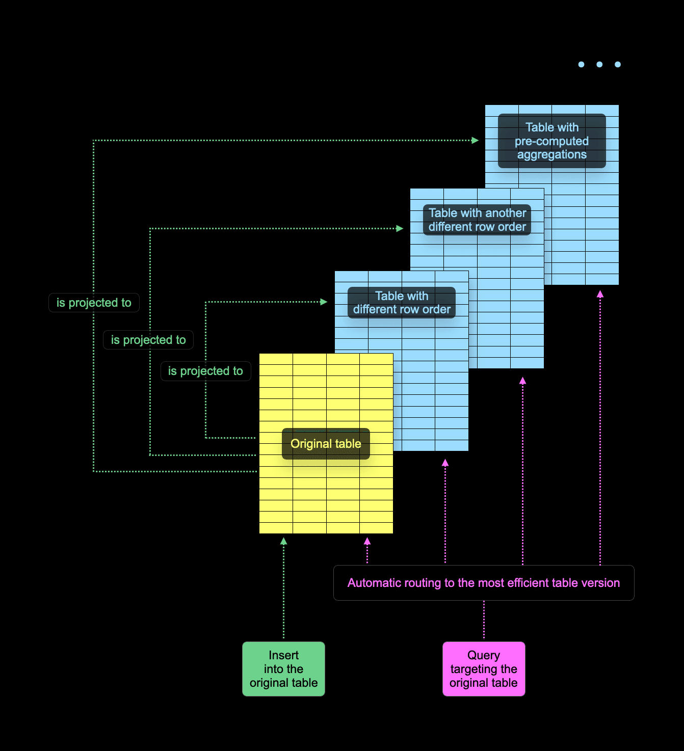
The decision to read from the original table or one of its projections is made individually per every table part. ClickHouse generally aims to read as little data as possible and employs a couple of tricks to identify the best part to read from, for example, sampling the primary key of a part. In some cases, source table parts have no corresponding projection parts. This can happen, for example, because creating a projection for a table in SQL is “lazy” by default - it only affects newly inserted data but keeps existing parts unaltered.

The following diagram shows a more concrete example of a query that computes the maximum price of properties sold in the U.K. grouped by town and street:

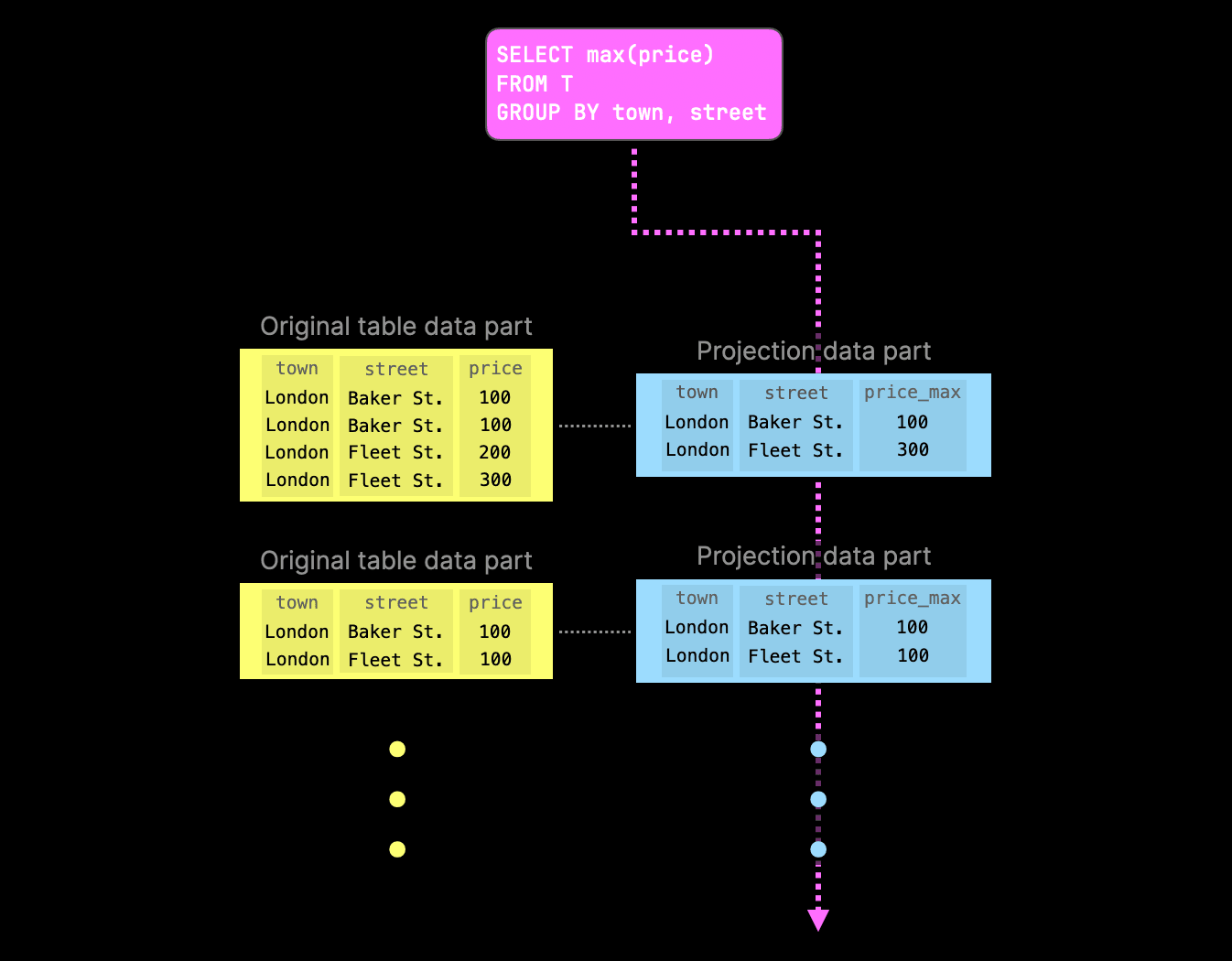
As one of the projections already contains the pre-computed aggregate values, ClickHouse tries to read from the corresponding projection parts to avoid aggregating at query runtime again. If a specific part lacks the corresponding projection part, query execution falls back to the original part.

But what happens if the rows in the original table change in a non-trivial way by non-trivial data part background merges?

For example, assume the table is stored using ClickHouse’s ReplacingMergeTree table engine. If the same row is detected in multiple input parts during merge, only the most recent row version (from the most recently inserted part) will be kept, while all older versions will be discarded.

Similarly, if the table is stored using the AggregatingMergeTree table engine, the merge operation may fold the same rows in the input parts (based on the primary key values) into a single row to update partial aggregation states.

Before ClickHouse v24.8, projection parts either silently got out of sync with the main data, or certain operations like updates and deletes could not be run at all as the database automatically threw an exception if the table had projections.

Since v24.8, a new table-level setting deduplicate_merge_projection_mode controls the behavior if the aforementioned non-trivial background merge operations occur in parts of the original table.

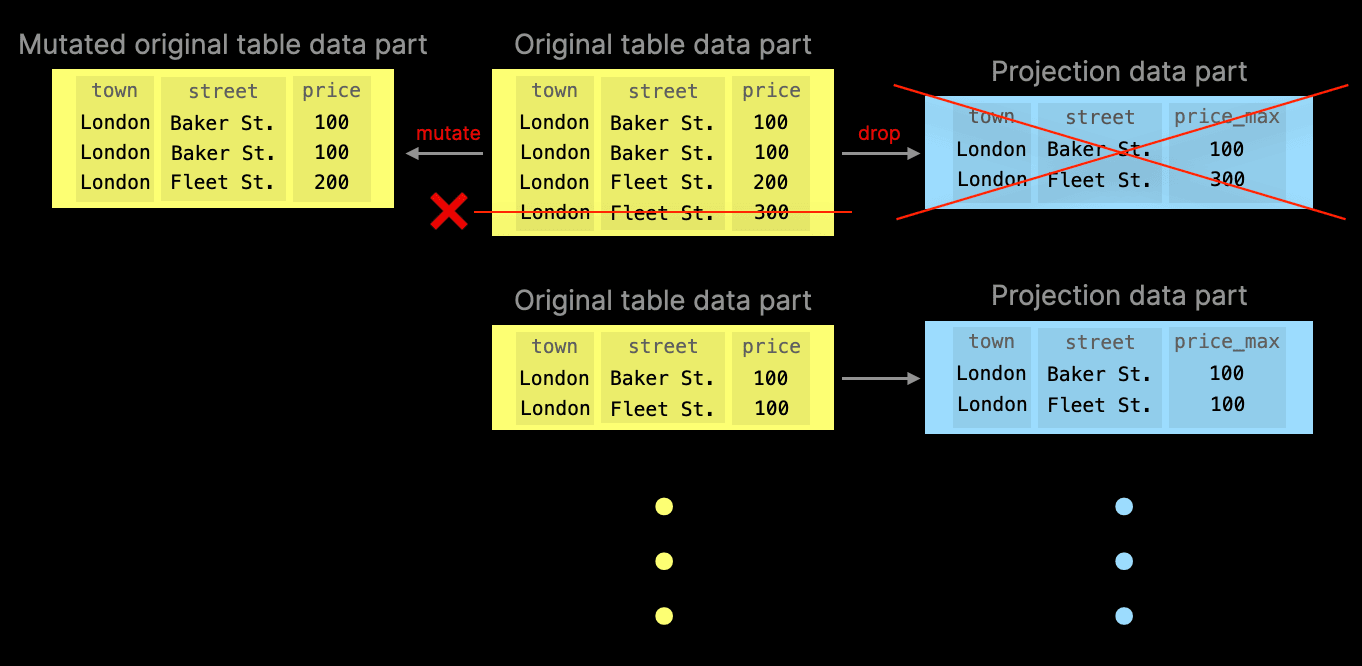
Delete mutations are another example of part merge operations that drop rows in the parts of the original table. Since v24.7, we also have a setting to control the behavior w.r.t. delete mutations triggered by lightweight deletes: lightweight_mutation_projection_mode.

Below are the possible values for both deduplicate_merge_projection_mode and lightweight_mutation_projection_mode:

• throw: an exception is thrown, preventing projection parts from going out of sync.

• drop: affected projection table parts are dropped. Queries will fall back to the original table part for affected projection parts.

• rebuild: the affected projection part is rebuilt to stay consistent with data in the original table part.

We demonstrate the drop behavior with two diagrams. The first diagram shows a row in the original table data part is deleted (by running a mutation merge operation). To prevent projection parts from becoming out-of-sync, the associated projection table data part is deleted:

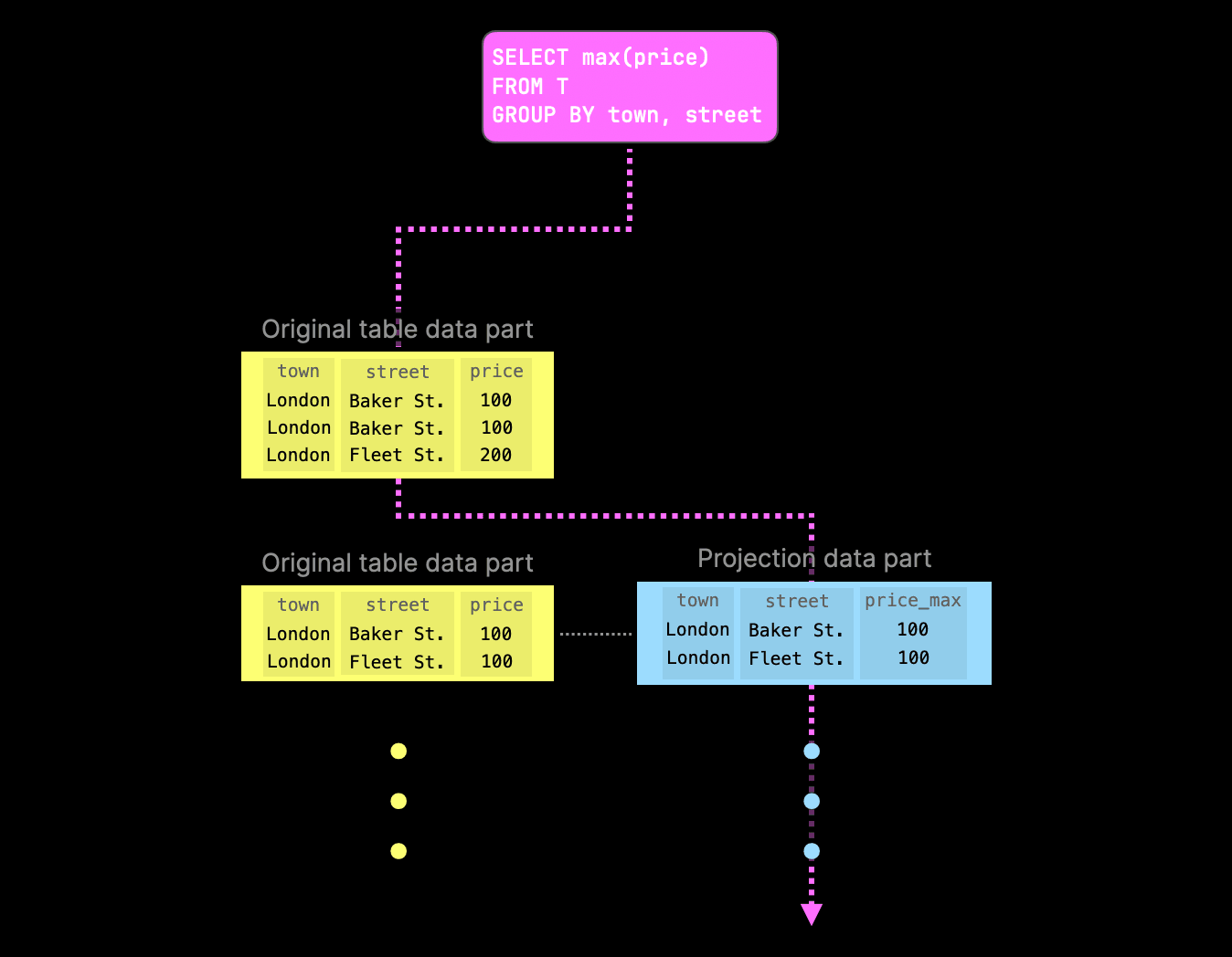
The example aggregation query would still be able to run (albeit slower) - it will simply fall back to the original table part for parts where it cannot find projection parts. However, when a projection part still exists, query execution would prefer these over the original table parts:

If deduplicate_merge_projection_mode is set to rebuild, ClickHouse will rebuild the projection table data part associated with the modified original table data part:

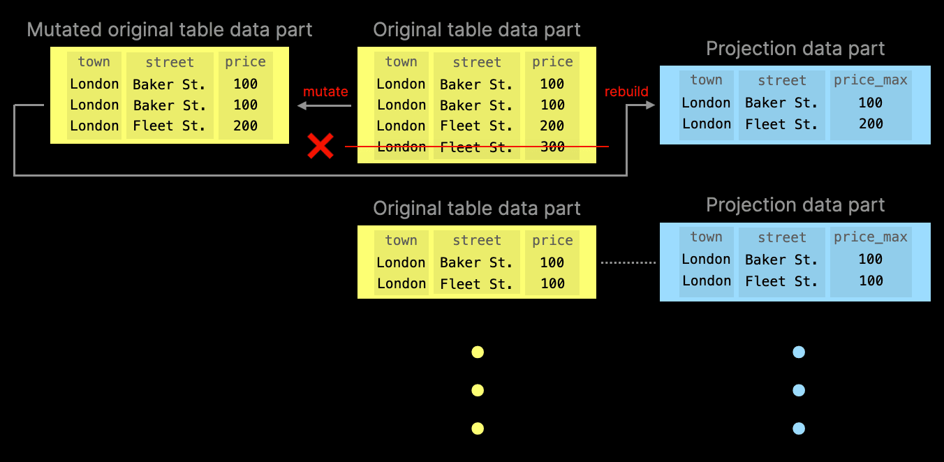
Note that this behavior is a significant advantage over incremental materialized views, which are similar to projections. However, incremental materialized views only react and sync on data inserts in the original table. When the original table data is updated, deleted, replaced, etc., the materialized views go (silently) out of sync.

This release also introduces the TimeSeries table engine. This table engine lets you use ClickHouse as the storage for Prometheus using the remote-write protocol. Prometheus can also query the data from ClickHouse using the remote-read protocol, as shown in the diagram below.

The TimeSeries table engine is an experimental feature, so you must set the allow_experimental_time_series_table property to enable it. We’re going to do that via a server config file:

config.d/allow_experimental_time_series.xml

<clickhouse>
    <profiles>
        <default>
            <allow_experimental_time_series_table>1</allow_experimental_time_series_table>
        </default>
    </profiles>
</clickhouse>

We’ll also need to set up some other configuration to enable the remove-write and remote-read endpoints in ClickHouse.

config.d/prometheus.xml

<clickhouse>
    <prometheus>
        <port>9092</port>
        <handlers>
            <my_rule_1>
                <url>/write</url>
                <handler>
                    <type>remote_write</type>
                    <table>default.prometheus</table>
                </handler>
            </my_rule_1>
            <my_rule_2>
                <url>/read</url>
                <handler>
                    <type>remote_read</type>
                    <table>default.prometheus</table>
                </handler>
            </my_rule_2>
        </handlers>
    </prometheus>
</clickhouse>

We can then start ClickHouse. We should see the following lines in the log output:

2024.08.27 15:41:19.970465 [ 14489686 ] {} <Information> Application: Listening for Prometheus: http://[::1]:9092
...
2024.08.27 15:41:19.970523 [ 14489686 ] {} <Information> Application: Listening for Prometheus: http://127.0.0.1:9092

Next, we’ll connect to the server using ClickHouse Client and run the following query:

CREATE TABLE prometheus ENGINE=TimeSeries;

Running this query will create three target tables:

• data, which contains time series associated with some identifier
• tags, which contains identifiers calculated for each combination of a metric name and tags.
• metrics, which contains some information about metrics that have been collected, the types of those metrics, and their descriptions.

You can see the names of those tables by running the following query:

SHOW TABLES

┌─name───────────────────────────────────────────────────┐
│ .inner_id.data.bcd5b4e6-01d3-45d1-ab27-bbe9de2bc74b    │
│ .inner_id.metrics.bcd5b4e6-01d3-45d1-ab27-bbe9de2bc74b │
│ .inner_id.tags.bcd5b4e6-01d3-45d1-ab27-bbe9de2bc74b    │
│ prometheus                                             │
└────────────────────────────────────────────────────────┘

Let’s now run Prometheus and have it collect data about itself in an extremely meta way. We’ll have the following configuration file:

prometheus.yml

global:
  scrape_interval:     15s
  external_labels:
    monitor: 'codelab-monitor'

scrape_configs:
  - job_name: 'prometheus'
    scrape_interval: 5s
    static_configs:
      - targets: ['localhost:9090']      

remote_write:
  - url: "http://localhost:9092/write"

remote_read:
  - url: "http://localhost:9092/read"

The important parts to note are remote_write and remote_read, which point to HTTP endpoints running on the ClickHouse Server. You can download Prometheus, and after you’ve unpacked the tar/zip file, run the following (or similar):

./prometheus-2.54.0.darwin-amd64/prometheus --config prometheus.yml

We can then look at the metrics in Prometheus, or there are some table functions that we can use in ClickHouse. They have the prefix timeSeries and take the ``TimeSeries table name as an argument. The first one is timeSeriesMetrics, which lists all the metrics:

SELECT *
FROM timeSeriesMetrics(prometheus)
LIMIT 3
FORMAT Vertical

Query id: 07f4cce2-ad47-45e1-b0e3-6903e474d76c

Row 1:
──────
metric_family_name: go_gc_cycles_automatic_gc_cycles_total
type:               counter
unit:
help:               Count of completed GC cycles generated by the Go runtime.

Row 2:
──────
metric_family_name: go_gc_cycles_forced_gc_cycles_total
type:               counter
unit:
help:               Count of completed GC cycles forced by the application.

Row 3:
──────
metric_family_name: go_gc_cycles_total_gc_cycles_total
type:               counter
unit:
help:               Count of all completed GC cycles.

We also have timeSeriesData and timeSeriesTags, which are best queried together:

SELECT *
FROM timeSeriesData(prometheus) AS data
INNER JOIN timeSeriesTags(prometheus) AS tags ON tags.id = data.id
WHERE metric_name = 'prometheus_tsdb_head_chunks_created_total'
LIMIT 1
FORMAT Vertical

Row 1:
──────
id:          a869dbe8-ba86-1416-47d3-c51cda7334b1
timestamp:   2024-08-27 15:54:46.655
value:       8935
tags.id:     a869dbe8-ba86-1416-47d3-c51cda7334b1
metric_name: prometheus_tsdb_head_chunks_created_total
tags:        {'instance':'localhost:9090','job':'prometheus','monitor':'codelab-monitor'}
min_time:    2024-08-27 13:46:05.725
max_time:    2024-08-27 16:00:26.649

In future versions, we will also implement the /query endpoint so you can do Prometheus-style queries directly against ClickHouse.

Since every ClickHouse release includes JOIN improvements, ClickHouse v24.8 is no exception, delivering even more enhancements.

ClickHouse v24.5 introduced experimental support for non-equal conditions in the ON clause of a JOIN. This release supports more join strictnesses (LEFT/RIGHT SEMI/ANTI/ANY JOIN) with unequal conditions involving columns from both the left and right tables.

ClickHouse tables with a join table engine contain an in-memory pre-computed hash table with the right-hand side table data ready for JOINs.

In ClickHouse v24.8, you can now run an OPTIMIZE TABLE statement on a Join table, which will lower memory usage by better packing. This can reduce the table memory footprint by 30%.

We also have a new experimental Kafka engine. This version makes it possible to have exactly- once processing of messages from Kafka.

In the existing engine, Kafka offsets are stored in Kafka and ClickHouse via a non-atomic commit. This leads to the possibility of duplicates in the case of retries.

In the new version, offsets are handled by ClickHouse Keeper. If an insertion attempt fails, it will take the same chunk of data and repeat the insertion, regardless of network or server failures.

We can enable the new engine by using these settings:

CREATE TABLE ... ENGINE = Kafka(
    'localhost:19092', 'topic', 'consumer', 'JSONEachRow')
SETTINGS
    kafka_keeper_path = '/clickhouse/{database}/kafka',
    kafka_replica_name = 'r1';