Blog / Engineering

ClickHouse Release 24.5

The ClickHouse Team

Jun 5, 2024

ClickHouse version 24.5 contains 19 new features 🎁 20 performance optimisations 🛷 68 bug fixes 🐛

As always, we send a special welcome to all the new contributors in 24.5! ClickHouse's popularity is, in large part, due to the efforts of the community that contributes. Seeing that community grow is always humbling.

Below are the names of the new contributors:

Alex Katsman, Alexey Petrunyaka, Ali, Caio Ricciuti, Danila Puzov, Evgeniy Leko, Francisco Javier Jurado Moreno, Gabriel Martinez, Grégoire Pineau, KenL, Leticia Webb, Mattias Naarttijärvi, Maxim Alexeev, Michael Stetsyuk, Pazitiff9, Sariel, TTPO100AJIEX, Tomer Shafir, Vinay Suryadevara, Volodya, Volodya Giro, Volodyachan, Xiaofei Hu, ZhiHong Zhang, Zimu Li, anonymous, [email protected], p1rattttt, pet74alex, qiangxuhui, sarielwxm, v01dxyz, vinay92-ch, woodlzm, zhou, zzyReal666

Hint: if you’re curious how we generate this list… click here.

You can also view the slides from the presentation.

This release introduces a new experimental data type for semi-structured data. The Dynamic data type is similar to the Variant data type introduced in version 24.1, but you don’t have to specify the accepted data types upfront.

For example, if we wanted to allow String, UInt64, and Array(String) values, we’d need to define a Variant(String, UInt64, Array(String)) column type. The equivalent for the dynamic data type would be Dynamic, and we could add values of any other types if we wanted to.

If you want to use this data type, you’ll need to set the following config parameter:

SET allow_experimental_dynamic_type = 1;

Suppose we have a file, sensors.json, containing sensor readings. The readings haven’t been collected consistently, meaning we have a mixture of types of values.

{"sensor_id": 1, "reading_time": "2024-06-05 12:00:00", "reading": 23.5}
{"sensor_id": 2, "reading_time": "2024-06-05 12:05:00", "reading": "OK"}
{"sensor_id": 3, "reading_time": "2024-06-05 12:10:00", "reading": 100}
{"sensor_id": 4, "reading_time": "2024-06-05 12:15:00", "reading": "62F"}
{"sensor_id": 5, "reading_time": "2024-06-05 12:20:00", "reading": 45.7}
{"sensor_id": 6, "reading_time": "2024-06-05 12:25:00", "reading": "ERROR"}
{"sensor_id": 7, "reading_time": "2024-06-05 12:30:00", "reading": "22.5C"}

This looks like a good use case for the Dynamic type, so let’s create a table:

CREATE TABLE sensor_readings (
    sensor_id UInt32,
    reading_time DateTime,
    reading Dynamic
) ENGINE = MergeTree()
ORDER BY (sensor_id, reading_time);

Now, we can run the following query to ingest the data:

INSERT INTO sensor_readings
select * FROM 'sensors.json';

Next, let’s query the table, returning all the columns, as well as the underlying types of the values stored in the reading column:

SELECT
    sensor_id,
    reading_time,
    reading,
    dynamicType(reading) AS type
FROM sensor_readings

Query id: eb6bf220-1c08-42d5-8e9d-1f77247897c3

   ┌─sensor_id─┬────────reading_time─┬─reading─┬─type────┐
1. │         1 │ 2024-06-05 12:00:00 │ 23.5    │ Float64 │
2. │         2 │ 2024-06-05 12:05:00 │ OK      │ String  │
3. │         3 │ 2024-06-05 12:10:00 │ 100     │ Int64   │
4. │         4 │ 2024-06-05 12:15:00 │ 62F     │ String  │
5. │         5 │ 2024-06-05 12:20:00 │ 45.7    │ Float64 │
6. │         6 │ 2024-06-05 12:25:00 │ ERROR   │ String  │
7. │         7 │ 2024-06-05 12:30:00 │ 22.5C   │ String  │
   └───────────┴─────────────────────┴─────────┴─────────┘

If we want only to retrieve the rows that use a specific type, we can use the dynamicElement function or the equivalent dot syntax:

SELECT
    sensor_id, reading_time, 
    dynamicElement(reading, 'Float64') AS f1, 
    reading.Float64 AS f2,
    dynamicElement(reading, 'Int64') AS f3, 
    reading.Int64 AS f4
FROM sensor_readings;

Query id: add6fbca-6dcd-4413-9f1f-0566c94c1aab

   ┌─sensor_id─┬────────reading_time─┬───f1─┬───f2─┬───f3─┬───f4─┐
1. │         1 │ 2024-06-05 12:00:00 │ 23.5 │ 23.5 │ ᴺᵁᴸᴸ │ ᴺᵁᴸᴸ │
2. │         2 │ 2024-06-05 12:05:00 │ ᴺᵁᴸᴸ │ ᴺᵁᴸᴸ │ ᴺᵁᴸᴸ │ ᴺᵁᴸᴸ │
3. │         3 │ 2024-06-05 12:10:00 │ ᴺᵁᴸᴸ │ ᴺᵁᴸᴸ │  100 │  100 │
4. │         4 │ 2024-06-05 12:15:00 │ ᴺᵁᴸᴸ │ ᴺᵁᴸᴸ │ ᴺᵁᴸᴸ │ ᴺᵁᴸᴸ │
5. │         5 │ 2024-06-05 12:20:00 │ 45.7 │ 45.7 │ ᴺᵁᴸᴸ │ ᴺᵁᴸᴸ │
6. │         6 │ 2024-06-05 12:25:00 │ ᴺᵁᴸᴸ │ ᴺᵁᴸᴸ │ ᴺᵁᴸᴸ │ ᴺᵁᴸᴸ │
7. │         7 │ 2024-06-05 12:30:00 │ ᴺᵁᴸᴸ │ ᴺᵁᴸᴸ │ ᴺᵁᴸᴸ │ ᴺᵁᴸᴸ │
   └───────────┴─────────────────────┴──────┴──────┴──────┴──────┘

If we want to compute the average of the reading column when the type is Int64 or Float64, we could write the following query:

SELECT avg(assumeNotNull(reading.Int64) + assumeNotNull(reading.Float64)) AS avg
FROM sensor_readings
WHERE dynamicType(reading) != 'String'

Query id: bb3fd8a6-07b3-4384-bd82-7515b7a1706f

   ┌──avg─┐
1. │ 56.4 │
   └──────┘

The Dynamic Type forms part of a longer-term project to add semi-structured columns to ClickHouse.

Since version 23.8, it’s been possible to read data from files inside archive files (e.g., zip/tar) as long as the archive files are on your local file system. In version 24.5, that functionality is extended to archive files that live on S3.

Let’s look at how it works by querying some ZIP files containing CSV files. We’ll start by writing a query that lists the embedded CSV files:

SELECT _path
FROM s3('s3://umbrella-static/top-1m-2024-01-*.csv.zip :: *.csv', One)
ORDER BY _path ASC

Query id: 07de510c-229f-4223-aeb9-b2cd36224228

    ┌─_path─────────────────────────────────────────────────┐
 1. │ umbrella-static/top-1m-2024-01-01.csv.zip::top-1m.csv │
 2. │ umbrella-static/top-1m-2024-01-02.csv.zip::top-1m.csv │
 3. │ umbrella-static/top-1m-2024-01-03.csv.zip::top-1m.csv │
 4. │ umbrella-static/top-1m-2024-01-04.csv.zip::top-1m.csv │
 5. │ umbrella-static/top-1m-2024-01-05.csv.zip::top-1m.csv │
 6. │ umbrella-static/top-1m-2024-01-06.csv.zip::top-1m.csv │
 7. │ umbrella-static/top-1m-2024-01-07.csv.zip::top-1m.csv │
 8. │ umbrella-static/top-1m-2024-01-08.csv.zip::top-1m.csv │
 9. │ umbrella-static/top-1m-2024-01-09.csv.zip::top-1m.csv │
10. │ umbrella-static/top-1m-2024-01-10.csv.zip::top-1m.csv │
11. │ umbrella-static/top-1m-2024-01-11.csv.zip::top-1m.csv │
12. │ umbrella-static/top-1m-2024-01-12.csv.zip::top-1m.csv │
13. │ umbrella-static/top-1m-2024-01-13.csv.zip::top-1m.csv │
14. │ umbrella-static/top-1m-2024-01-14.csv.zip::top-1m.csv │
15. │ umbrella-static/top-1m-2024-01-15.csv.zip::top-1m.csv │
16. │ umbrella-static/top-1m-2024-01-16.csv.zip::top-1m.csv │
17. │ umbrella-static/top-1m-2024-01-17.csv.zip::top-1m.csv │
18. │ umbrella-static/top-1m-2024-01-18.csv.zip::top-1m.csv │
19. │ umbrella-static/top-1m-2024-01-19.csv.zip::top-1m.csv │
20. │ umbrella-static/top-1m-2024-01-20.csv.zip::top-1m.csv │
21. │ umbrella-static/top-1m-2024-01-21.csv.zip::top-1m.csv │
22. │ umbrella-static/top-1m-2024-01-22.csv.zip::top-1m.csv │
23. │ umbrella-static/top-1m-2024-01-23.csv.zip::top-1m.csv │
24. │ umbrella-static/top-1m-2024-01-24.csv.zip::top-1m.csv │
25. │ umbrella-static/top-1m-2024-01-25.csv.zip::top-1m.csv │
26. │ umbrella-static/top-1m-2024-01-26.csv.zip::top-1m.csv │
27. │ umbrella-static/top-1m-2024-01-27.csv.zip::top-1m.csv │
28. │ umbrella-static/top-1m-2024-01-28.csv.zip::top-1m.csv │
29. │ umbrella-static/top-1m-2024-01-29.csv.zip::top-1m.csv │
30. │ umbrella-static/top-1m-2024-01-30.csv.zip::top-1m.csv │
31. │ umbrella-static/top-1m-2024-01-31.csv.zip::top-1m.csv │
    └───────────────────────────────────────────────────────┘

So, we have 31 files to work with. Let’s next compute how many rows of data there are across those files:

SELECT
    _path,
    count()
FROM s3('s3://umbrella-static/top-1m-2024-01-*.csv.zip :: *.csv', CSV)
GROUP BY _path

Query id: 07de510c-229f-4223-aeb9-b2cd36224228

    ┌─_path─────────────────────────────────────────────────┬─count()─┐
 1. │ umbrella-static/top-1m-2024-01-21.csv.zip::top-1m.csv │ 1000000 │
 2. │ umbrella-static/top-1m-2024-01-07.csv.zip::top-1m.csv │ 1000000 │
 3. │ umbrella-static/top-1m-2024-01-30.csv.zip::top-1m.csv │ 1000000 │
 4. │ umbrella-static/top-1m-2024-01-16.csv.zip::top-1m.csv │ 1000000 │
 5. │ umbrella-static/top-1m-2024-01-10.csv.zip::top-1m.csv │ 1000000 │
 6. │ umbrella-static/top-1m-2024-01-27.csv.zip::top-1m.csv │ 1000000 │
 7. │ umbrella-static/top-1m-2024-01-01.csv.zip::top-1m.csv │ 1000000 │
 8. │ umbrella-static/top-1m-2024-01-29.csv.zip::top-1m.csv │ 1000000 │
 9. │ umbrella-static/top-1m-2024-01-13.csv.zip::top-1m.csv │ 1000000 │
10. │ umbrella-static/top-1m-2024-01-24.csv.zip::top-1m.csv │ 1000000 │
11. │ umbrella-static/top-1m-2024-01-02.csv.zip::top-1m.csv │ 1000000 │
12. │ umbrella-static/top-1m-2024-01-22.csv.zip::top-1m.csv │ 1000000 │
13. │ umbrella-static/top-1m-2024-01-18.csv.zip::top-1m.csv │ 1000000 │
14. │ umbrella-static/top-1m-2024-01-04.csv.zip::top-1m.csv │ 1000001 │
15. │ umbrella-static/top-1m-2024-01-15.csv.zip::top-1m.csv │ 1000000 │
16. │ umbrella-static/top-1m-2024-01-09.csv.zip::top-1m.csv │ 1000000 │
17. │ umbrella-static/top-1m-2024-01-06.csv.zip::top-1m.csv │ 1000000 │
18. │ umbrella-static/top-1m-2024-01-20.csv.zip::top-1m.csv │ 1000000 │
19. │ umbrella-static/top-1m-2024-01-17.csv.zip::top-1m.csv │ 1000000 │
20. │ umbrella-static/top-1m-2024-01-31.csv.zip::top-1m.csv │ 1000000 │
21. │ umbrella-static/top-1m-2024-01-11.csv.zip::top-1m.csv │ 1000000 │
22. │ umbrella-static/top-1m-2024-01-26.csv.zip::top-1m.csv │ 1000000 │
23. │ umbrella-static/top-1m-2024-01-12.csv.zip::top-1m.csv │ 1000000 │
24. │ umbrella-static/top-1m-2024-01-28.csv.zip::top-1m.csv │ 1000000 │
25. │ umbrella-static/top-1m-2024-01-03.csv.zip::top-1m.csv │ 1000001 │
26. │ umbrella-static/top-1m-2024-01-25.csv.zip::top-1m.csv │ 1000000 │
27. │ umbrella-static/top-1m-2024-01-05.csv.zip::top-1m.csv │ 1000000 │
28. │ umbrella-static/top-1m-2024-01-19.csv.zip::top-1m.csv │ 1000000 │
29. │ umbrella-static/top-1m-2024-01-23.csv.zip::top-1m.csv │ 1000000 │
30. │ umbrella-static/top-1m-2024-01-08.csv.zip::top-1m.csv │ 1000000 │
31. │ umbrella-static/top-1m-2024-01-14.csv.zip::top-1m.csv │ 1000000 │
    └───────────────────────────────────────────────────────┴─────────┘

We have more or less 1 million rows per file. Let’s have a look at some of the rows. We can use the DESCRIBE clause to understand the structure of the data:

DESCRIBE TABLE s3('s3://umbrella-static/top-1m-2024-01-*.csv.zip :: *.csv', CSV)
SETTINGS describe_compact_output = 1

Query id: d5afed03-6c51-40f4-b457-1065479ef1a8

   ┌─name─┬─type─────────────┐
1. │ c1   │ Nullable(Int64)  │
2. │ c2   │ Nullable(String) │
   └──────┴──────────────────┘

Finally, let’s have a look at a few of the rows themselves:

SELECT *
FROM s3('s3://umbrella-static/top-1m-2024-01-*.csv.zip :: *.csv', CSV)
LIMIT 5

Query id: bd0d9bd9-19cb-4b2e-9f63-6b8ffaca85b1

   ┌─c1─┬─c2────────────────────────┐
1. │  1 │ google.com                │
2. │  2 │ microsoft.com             │
3. │  3 │ data.microsoft.com        │
4. │  4 │ events.data.microsoft.com │
5. │  5 │ netflix.com               │
   └────┴───────────────────────────┘

The previous release already brought significant JOIN performance improvements. From now on, you will actually see JOIN improvements in every ClickHouse release. 🚀

In this release, we focused on improving the memory usage of the CROSS JOIN.

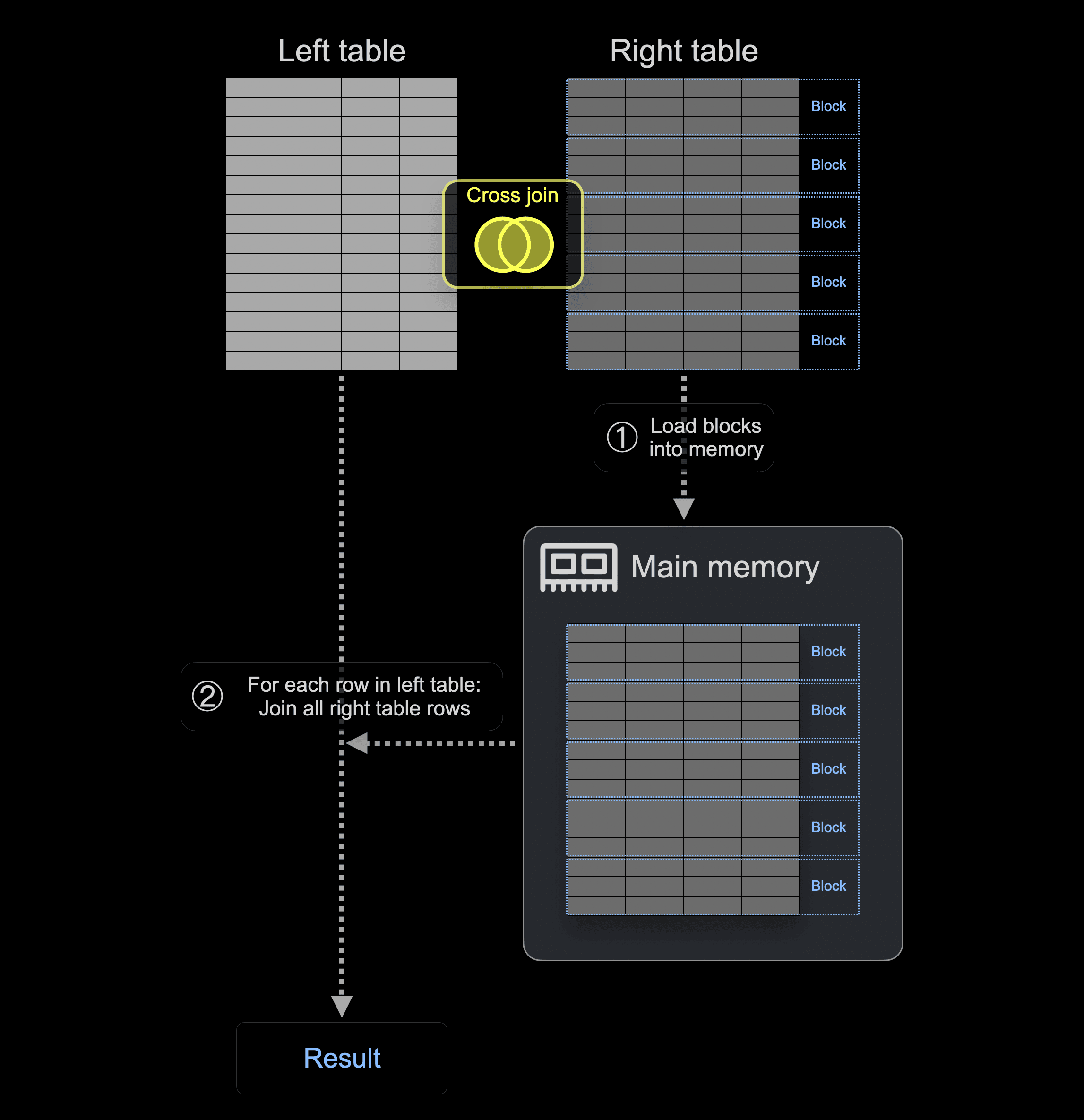
As a reminder, the CROSS JOIN produces the full cartesian product of two tables without considering join keys. Meaning that each row from the left table is combined with each row from the right table.

For that reason, CROSS join is implemented without utilizing hash tables. Instead, ① ClickHouse loads all blocks from the right table into the main memory, and then, ② for each row in the left table, all right table rows are joined:

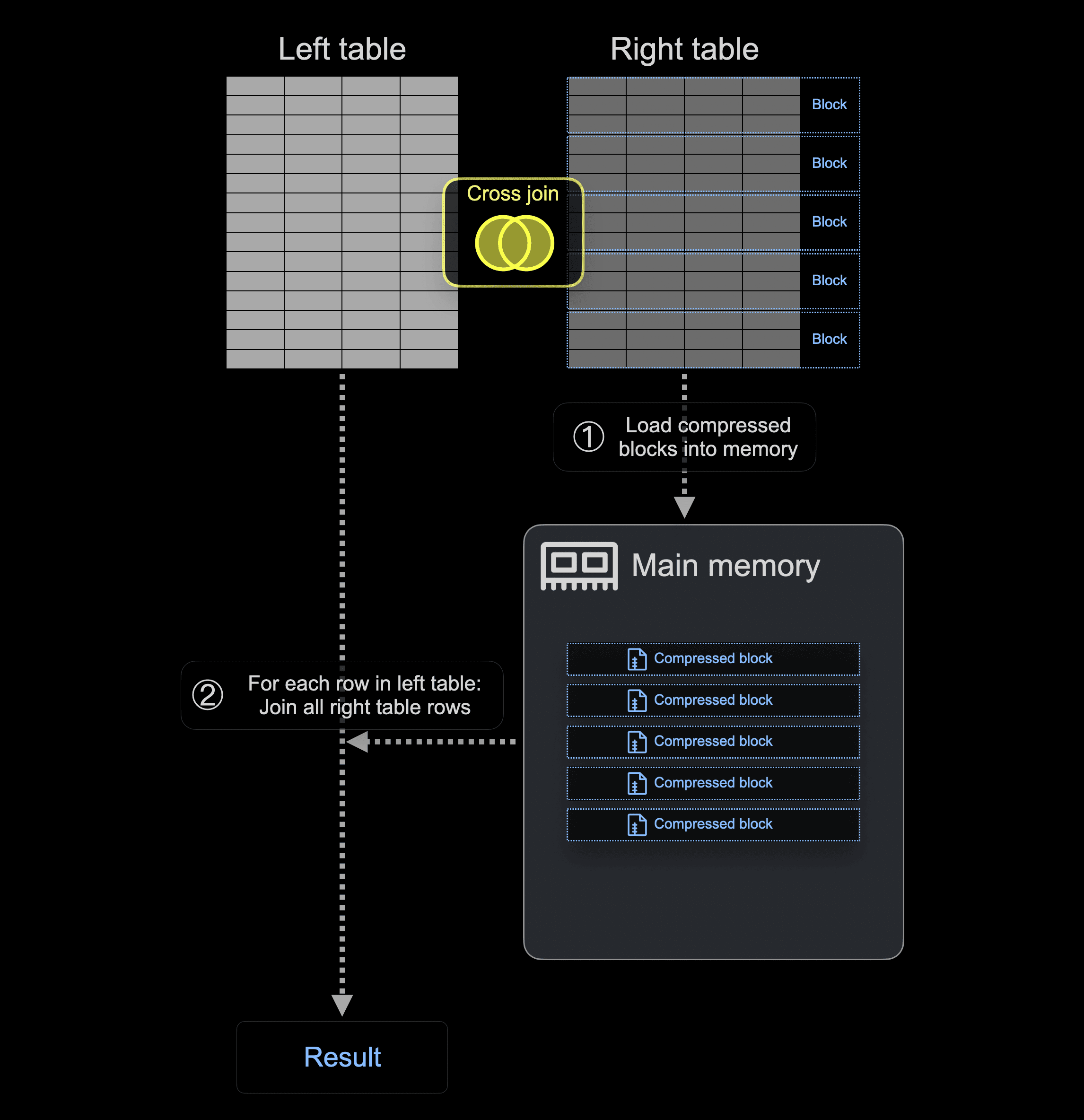
Now, with ClickHouse 24.5, the blocks from the right table can optionally be loaded into the main memory in compressed (LZ4) format or temporarily written to disk if they don’t fit into the memory.

The following diagram shows how, based on two new threshold settings - cross_join_min_rows_to_compress and cross_join_min_bytes_to_compress - ClickHouse loads compressed (LZ4) right table blocks into the main memory before executing the CROSS join:

To demonstrate this, we load 1 billion rows from the public PyPI download statistics into a table in both ClickHouse 24.4 and 24.5:

CREATE TABLE pypi_1b
(
    `timestamp` DateTime,
    `country_code` LowCardinality(String),
    `url` String,
    `project` String
)
ORDER BY (country_code, project, url, timestamp);

INSERT INTO pypi_1b
SELEC timestamp, country_code, url, project
FROM s3('https://storage.googleapis.com/clickhouse_public_datasets/pypi/file_downloads/sample/2023/{0..61}-*.parquet');

Now, we run a CROSS JOIN with ClickHouse 24.4. Note that we use an ad-hoc table with one row as the left table, as we are only interested in seeing the memory consumption of loading the right table rows into the main memory:

SELECT
    country_code,
    project
FROM
(
    SELECT 1
) AS L, pypi_1b AS R
ORDER BY (country_code, project) DESC
LIMIT 1000
FORMAT Null;

0 rows in set. Elapsed: 59.186 sec. Processed 1.01 billion rows, 20.09 GB (17.11 million rows/s., 339.42 MB/s.)
Peak memory usage: 51.77 GiB.

ClickHouse used 51.77 GiB of main memory for running this CROSS JOIN.

We run the same CROSS JOIN with ClickHouse 24.5 but with disabled compression (by setting the compression thresholds to 0):

SELECT
    country_code,
    project
FROM
(
    SELECT 1
) AS L, pypi_1b AS R
ORDER BY (country_code, project) DESC
LIMIT 1000
FORMAT Null
SETTINGS 
    cross_join_min_bytes_to_compress = 0, 
    cross_join_min_rows_to_compress = 0;

0 rows in set. Elapsed: 39.419 sec. Processed 1.01 billion rows, 20.09 GB (25.69 million rows/s., 509.63 MB/s.)
Peak memory usage: 19.06 GiB.

As you can see, in version 24.5, the memory usage for CROSS JOIN is optimized even without compression of the right table blocks: ClickHouse used 19.06 GiB of main memory instead of 51.77 GiB for the query above. In addition, the CROSS JOIN runs 20 seconds faster than with the previous version.

Finally, we run the example CROSS JOIN with ClickHouse 24.5 and (by default) enabled compression:

SELECT
    country_code,
    project
FROM
(
    SELECT 1
) AS L, pypi_1b AS R
ORDER BY (country_code, project) DESC
LIMIT 1000
FORMAT Null;

0 rows in set. Elapsed: 69.311 sec. Processed 1.01 billion rows, 20.09 GB (14.61 million rows/s., 289.84 MB/s.)
Peak memory usage: 5.36 GiB.

Because the row count or data size of the right table are above the cross_join_min_rows_to_compress or cross_join_min_bytes_to_compress thresholds, ClickHouse is loading the blocks from the right table compressed with LZ4 into memory, resulting in 5.36 GiB memory usage, which is ~ 10 times less memory usage compared to running the CROSS JOIN in 24.4. Note that the compression overhead increases the query's runtime.

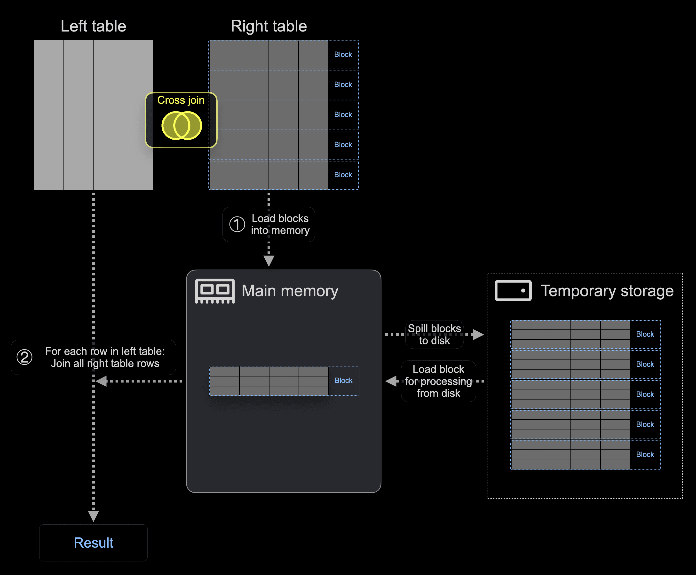
In addition, since this release, if the size of the right table blocks exceeds the max_bytes_in_join or max_rows_in_join thresholds, then ClickHouse spills the right table blocks from memory to disk:

We demonstrate this by running our example CROSS JOIN with ClickHouse 24.5 and enabled test level logging level. Note that we disabled compression and used a limited max_rows_in_join value to enforce the spilling of the right table blocks to disk:

./clickhouse client --send_logs_level=test --query "
SELECT
    country_code,
    project
FROM
(
    SELECT 1
) AS L, pypi_1b AS R
ORDER BY (country_code, project) DESC
LIMIT 1000
FORMAT Null
SETTINGS
    cross_join_min_rows_to_compress=0,
    cross_join_min_bytes_to_compress=0,
    max_bytes_in_join=0,
    max_rows_in_join=10_000;
" 2> log.txt

When we inspect the generated log.txt file, we can see entries like this:

TemporaryFileStream: Writing to temporary file ./tmp/tmpe8c8a301-ee67-40c4-af9a-db8e9c170d0c

And also overall memory usage and runtime:

Peak memory usage (for query): 300.52 MiB.
Processed in 58.823 sec.

We can see that this query run has a very low memory usage of 300.52 MiB as only a subset of the right table blocks are held in memory at each point in time during CROSS JOIN processing.

Before version 24.5, ClickHouse only allowed equality conditions in the ON clause of JOINS.

As an example, we get an exception when we run this JOIN query with ClickHouse 24.4:

SELECT L.*, R.*
FROM pypi_1b AS L INNER JOIN pypi_1b AS R 
ON (L.country_code = R.country_code) AND (L.timestamp < R.timestamp)
LIMIT 10
FORMAT Null;

Received exception from server (version 24.4.1): … INVALID_JOIN_ON_EXPRESSION

Now, with version 24.5, ClickHouse has experimental support for non-equal conditions in the ON clause. Note that, for now, we need to enable the allow_experimental_join_condition setting for this:

SELECT
    L.*,
    R.*
FROM pypi_1b AS L
INNER JOIN pypi_1b AS R ON 
     L.country_code = R.country_code AND 
     L.timestamp < R.timestamp
LIMIT 10
FORMAT Null
SETTINGS
    allow_experimental_join_condition = 1;

Stay tuned for many more JOIN improvements in the coming releases!

That’s all for the 24.5 release. We’d love for you to join us for the 24.6 release call on 27 June. Make sure you register so that you’ll get all the details for the Zoom webinar.

Share this post