Welcome to the September edition of What's New in ClickStack - the open-source observability stack for ClickHouse. Each month, we highlight the latest updates across the stack, combining new ClickHouse capabilities with HyperDX UI enhancements to unlock fresh workflows, smarter visualizations, and a smoother experience.
This release introduces dashboard import/export, support for custom aggregations, and the ability to extend the configuration for the OTel collector. We’ve also delivered several performance improvements, including time-window chunking and better support for gauge metrics with the delta function.
New contributors #
Building an open-source observability stack is a team sport - and our community makes it possible. A big thank you to this month's new contributors! Every contribution, big or small, helps make ClickStack better for everyone.
@elizabetdev @brandon-pereira @pulpdrew
Import/export dashboards #
One of the most requested features from the community has arrived: you can now import and export dashboards in HyperDX. This makes it easier than ever to share dashboards with teammates or contribute them back to the wider community.
Dashboards can be exported as versioned JSON files, ensuring compatibility today while giving us the flexibility to evolve the format and add new functionality in the future.
Consider the following simple dashboard showing analytics on our public demo ClickPy. Exporting requires a simple click, producing a JSON file users can share.
Importing is equally simple. Users can simply create a new saved dashboard and import the JSON file. To ensure portability, when importing a dashboard you’ll need to map its data sources (logs, traces, or metrics) to those already defined in HyperDX, so all visualizations connect correctly.
Looking ahead, we believe this feature opens the door to out-of-the-box experiences. Expect to see official, ready-to-use dashboards (for example, monitoring NGINX, Kafka, Redis etc) that can be imported directly into your environment. Stay tuned as we begin developing these out in the coming months!
Custom collector configuration #
September introduces the ability to modify the OpenTelemetry Collector configuration distributed with ClickStack.
ClickStack is built from three core components: HyperDX as the visualization layer, ClickHouse as the analytics engine that stores and supports querying of observability data efficiently, and an opinionated distribution of the OTel Collector. The collector configuration is managed through HyperDX using OpAmp to ensure ingestion remains secure - by requiring the ingestion API key that HyperDX provides in the UI. While this model guarantees security and configuration consistency, it has historically made customization difficult for users.
To extend the configuration, users can now supply their own OTel Collector Yaml, which is merged with the base configuration delivered via OPAMP. The custom file should be mounted into the container at /etc/otelcol-contrib/custom.config.yaml.
For example, if you’re deploying ClickStack locally and want to monitor host system metrics or local log files, you previously had to run a second OTel Collector with the right configuration and forward data into ClickStack’s ingestion endpoint provided by its packaged collector.
With the new extension mechanism, you can simply define the extra receivers you need and mount the file into the container - enabling host metrics and logs to flow into your local deployment with a single command.
A receiver configuration for local monitoring would typically look something like the following.
Note that we also need to ensure we have the required pipelines to route the data from our receivers to the clickhouse exporter defined in the base configuration:
1# local-monitoring.yaml
2receivers:
3  filelog:
4    include:
5      - /var/host/log/**/*.log # Linux
6      - /var/host/log/syslog
7      - /var/host/log/messages
8      - /private/var/log/*.log # macOS
9      - /tmp/all_events.log # macos - see below
10    start_at: beginning # modify to collect new files only
11
12  hostmetrics:
13    collection_interval: 1s
14    scrapers:
15      cpu:
16        metrics:
17          system.cpu.time:
18            enabled: true
19          system.cpu.utilization:
20            enabled: true
21      memory:
22        metrics:
23          system.memory.usage:
24            enabled: true
25          system.memory.utilization:
26            enabled: true
27      filesystem:
28        metrics:
29          system.filesystem.usage:
30            enabled: true
31          system.filesystem.utilization:
32            enabled: true
33      paging:
34        metrics:
35          system.paging.usage:
36            enabled: true
37          system.paging.utilization:
38            enabled: true
39          system.paging.faults:
40            enabled: true
41      disk:
42      load:
43      network:
44      processes:
45
46service:
47  pipelines:
48    logs/host:
49      exporters:
50        - clickhouse
51      processors:
52        - memory_limiter
53        - transform
54        - batch
55      receivers: [filelog]
56    metrics/host:
57      exporters:
58        - clickhouse
59      processors:
60        - memory_limiter
61        - batch
62      receivers: [hostmetrics]
To include this in the OTel collector, we simply need to mount this file into our container when deploying ClickStack:
1docker run --name clickstack-o11y \
2  -p 8080:8080 -p 4317:4317 -p 4318:4318 \
3  -v "$(pwd)/local-monitoring.yaml:/etc/otelcol-contrib/custom.config.yaml:ro" \
4  -v /var/log:/var/host/log:ro \
5  -v /private/var/log:/private/var/log:ro \
6  --user 0:0 \
7  docker.hyperdx.io/hyperdx/hyperdx-all-in-one
In this example, we also mount paths from our local file system to ensure the collector can read our host log files. This is an example only and should not be used in production, as it grants the container root access to read our system metrics and log files.
When we log into HyperDX, we should immediately see our local logs and be able to explore metrics as shown in our local monitoring guide:
This simple example highlights how the feature improves the getting-started experience, but the same flexibility is critical at scale. Users may want to pull events from Kafka, open a syslog interface for log ingestion, or configure tail and head sampling for traces. In rare cases, users may even need to adjust the ClickHouse exporter configuration - particularly in high-throughput environments where additional tuning is required.
Custom aggregations #
Historically, HyperDX limited chart building to a small set of common aggregation types. These included min, max, mean, median, and percentiles like the 90th, 95th, and 99th. While they covered most use cases, they constrained more advanced analysis.
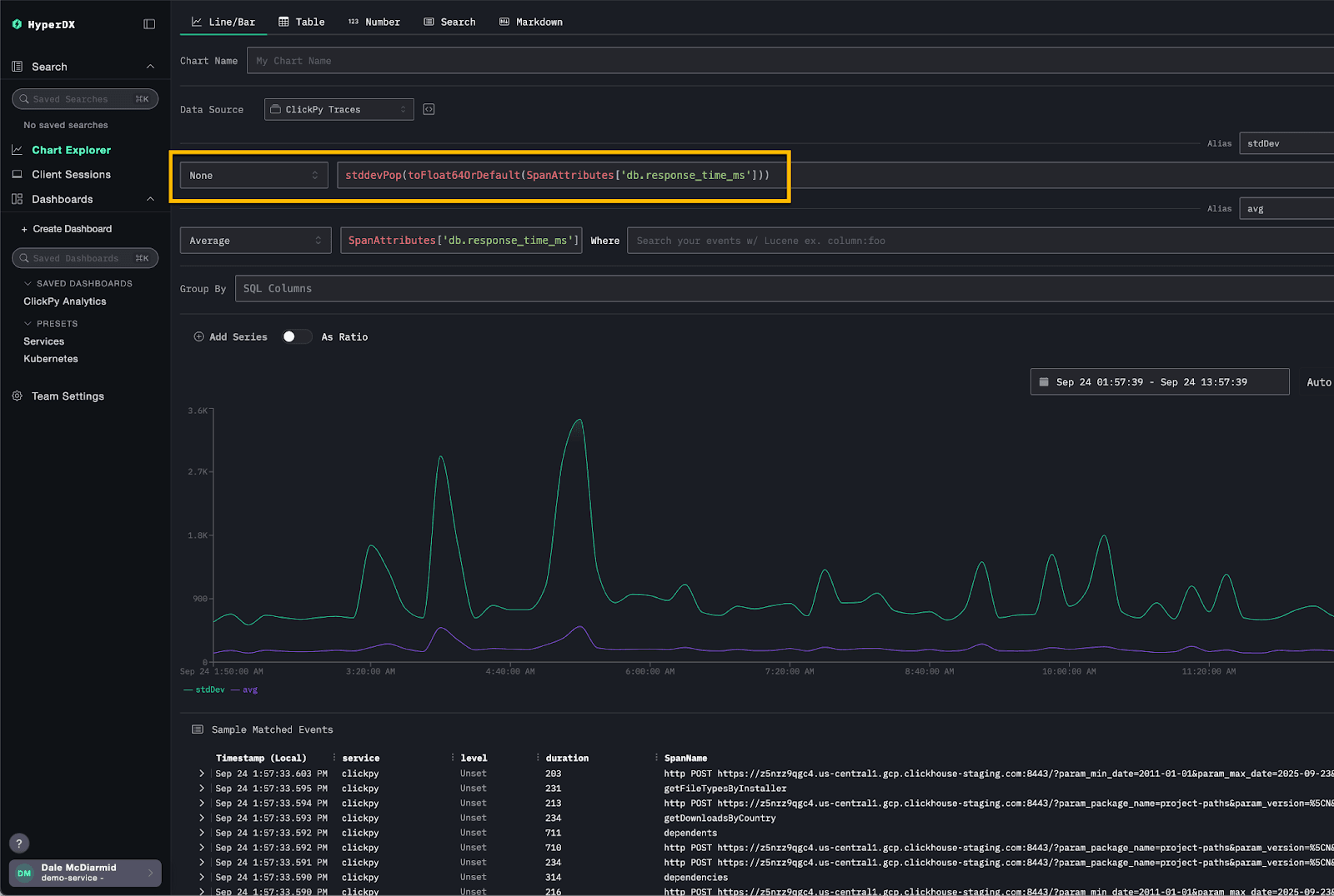
With the latest release, users can now unlock the full analytical capabilities of ClickHouse by selecting “none” as the aggregation type. This allows you to directly specify any ClickHouse aggregation function, exposing more than 100 analytical options for deeper and more flexible exploration of your data.
For example, consider the following visualization, which plots both the average response time and the variance for our ClickPy demo queries. Standard deviation can reveal fluctuations that an average alone might hide. While not exposed as a native option in HyperDX, it can be achieved by selecting “None” and using the stddevPop function directly as an expression.
Chunking time windows #
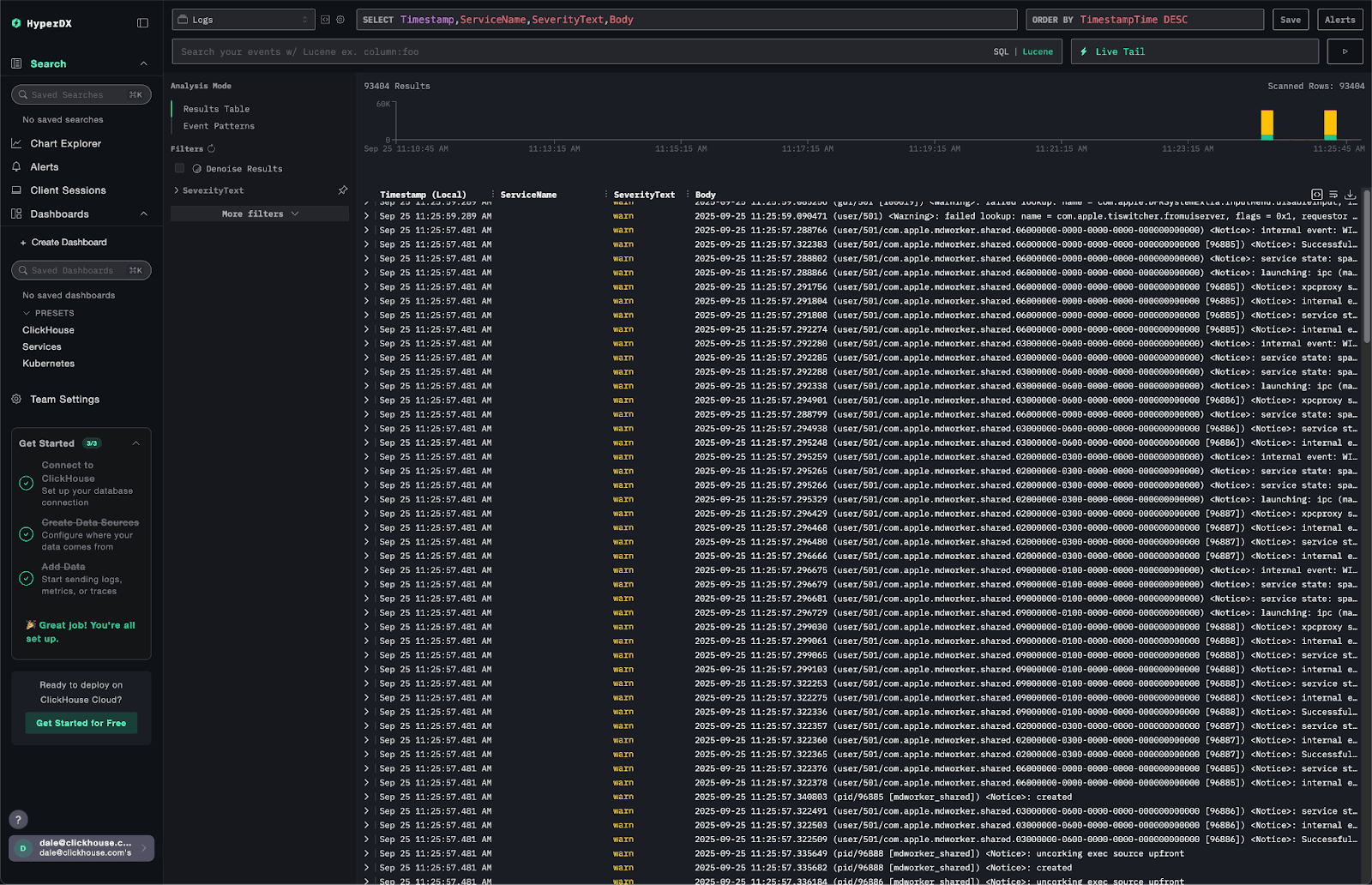
Previously, HyperDX executed a single query to load search results in the Search view. This was fine for smaller datasets or narrow time ranges, but it became inefficient at scale. Queries scanned the entire time window uniformly, rather than prioritizing resources to the recent data that users typically care about.
With the September release, HyperDX now chunks query execution by time window, starting with the most recent data. Subsequent windows are queried only if needed, and once the required number of results is reached, the remaining queries are canceled.
This approach prioritizes resources to deliver the freshest results first, while reducing overall execution time and system load.

Consider the above query over a four-hour time range. Instead of executing one large query, HyperDX splits it into sub-queries, each covering a smaller window. In this example, each query spans one hour: the first returns three results, the second adds two, and the third adds five. Because the interface only requires ten results, the final query is canceled.
In practice, HyperDX handles much larger time ranges and higher data volumes. By applying this chunking approach to search results, it ensures ClickHouse resources are focused on retrieving the most recent data first.
We are exploring how to apply this technique in other parts of HyperDX. For example, histogram views could be loaded asynchronously in chunks, allowing database resources to deliver quick responses and keep the interface interactive instead of forcing users to wait for results for the entire time range to complete.
Delta function #
The September release also adds support for applying a delta function to gauge metrics, matching the behavior of Prometheus’s delta() function.
A gauge is a metric that represents a single numerical value that can move up or down. Typical examples include system temperature, memory usage, or the number of concurrent requests. Unlike counters, which only increase until reset, gauges can fluctuate freely.
The delta() function basically aims to show you how much a gauge has changed over a given time window, adjusted so each window is comparable no matter when the samples landed.
The delta() function calculates the difference between the first and last value of a gauge within a time range window (the bucket or lookback range) e.g. [1m]. A new bucket is created at each evaluation step, covering the preceding range.
Note that the raw difference will be extrapolated to represent the full duration of the bucket, ensuring consistent comparisons across time windows. For example, if a one-minute bucket contains two points 30 seconds apart with a difference of 10, the result is scaled to 20 to represent the full minute.
Since each bucket may contain multiple series (distinguished by attributes such as host or service), multiple delta values can exist per bucket. The aggregation function (such as min, max, or avg) specified by the user is then applied across the deltas to produce the value displayed.
Examples of using delta() include tracking changes in pod memory usage. A positive delta consistently above zero indicates a pod’s memory footprint is steadily increasing, which can be an early sign of a memory leak and worth alerting on.
Consider the metric k8s.pod.memory.working_set above for the ClickHouse pod. Plotting the raw gauge value shows the absolute memory usage of a pod. By applying delta, you can instead visualize how much memory usage has changed within each interval. A sustained positive delta highlights the pod is steadily consuming more memory over time, while negative deltas indicate memory being released.