Get started with ClickHouse Cloud today and receive $300 in credits. To learn more about our volume-based discounts, contact us or visit our pricing page.
Table of Contents
Introduction
Over the past year, Large Language Models (LLMs) along with products like ChatGPT have captured the world's imagination and have been driving a new wave of functionality built on top of them. The concept of vectors and vector search is core to powering features like recommendations, question answering, image / video search, and much more.
As a result, we've seen a significant increase in vector search interest in our community. Specifically, an interest in better understanding when a specialized vector database becomes necessary, and when it doesn't.
With these models in focus, we take the opportunity to revisit search before vectors, explore what vectors (and embeddings) are, understand vector search, its applications, and how this functionality fits into the broader data landscape.
For those readers who are already familiar with the basic vector search concepts and want to jump straight to how vector search can be done in ClickHouse, you can find Part II here.
Search before vectors
Let’s briefly cover how search worked with traditional engines like Elasticsearch and Solr (note: these technologies now also offer vector search capabilities).
These engines focused on providing text search capabilities, relying on users breaking their content up into discrete units of text known as documents, each with an id. These documents could contain anything from all the text in a book or web page to a single sentence, depending on the granularity at which the user needed to find relevant content (length also impacts search effectiveness).
The text from each document would then be split into its component words through a process known as tokenization, which produces a bag of words. In its simplest form, tokenization would involve a sequential process of splitting on whitespace, lowercasing and removing punctuation. These words, also known as terms, would then be used to build an index similar to that found at the back of a book. This index would contain the count for every word in the text, the document ids in which they occurred, known as postings, as well as the count of how often each term occurred in a document.
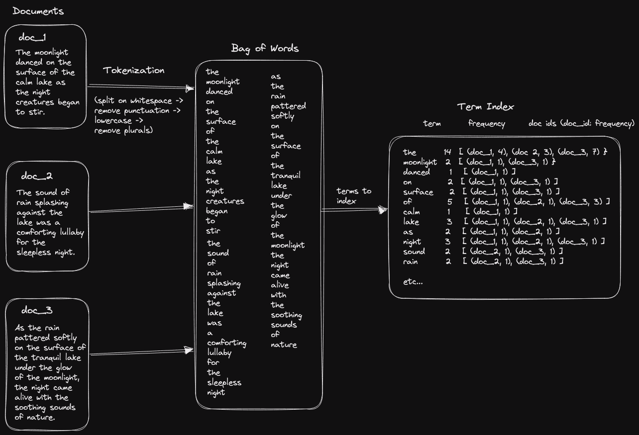
Note the above is a simplification and omits details on processes such as tokenization, stemming, lemmatization, and stop words, as well as positional indexes and the clever internal data structures used to deliver fast search.
When searching, the index would be accessed, and the matching documents identified. A calculation would then be performed for each document, comparing the search text to the document terms to order them for relevancy. This "relevancy calculation" was typically based on how often the matching terms occurred in the broader corpus and the document itself.
Words that were rare in the wider corpus, but common in the matching document, would contribute more to the document score than generically common words such as "and" which offer little meaning. These frequent words, referred to as "stop words", could be optionally omitted from the index given their low contribution to relevancy at some loss of features. This simple observation, made in the 1970s, formed the basis of the Term Frequency/Inverse Document Frequency (TF/IDF) formula, which, while simple, was often effective.
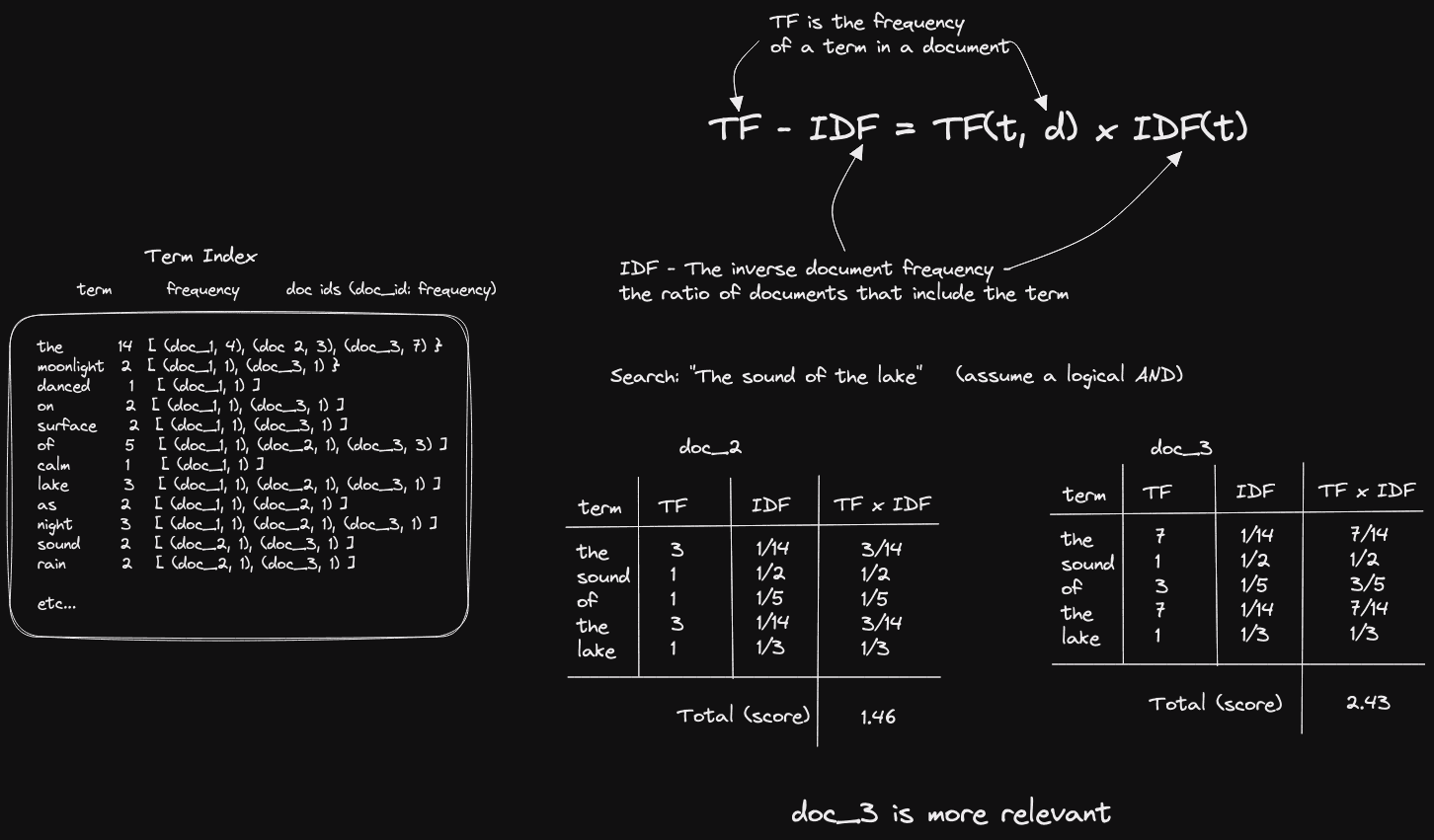
The above is a simplification. It assumes a logical AND between the terms, and the scores for each term are simply summed. Multi-term searches can be less restrictive, e.g., OR, utilize far more elaborate scoring functions, such as BM25, and methods for combining term scores.
The challenge with this approach is it fails to capture the meaning or context of the words themselves. Positional information could weigh documents more highly if the search terms were close, but this still fails to capture the semantic relationship between them. For example, this approach can't distinguish between:
"The cat watched the bird through the window with interest" and "The bird watched the cat through the window with interest."
Additionally, this approach suffers from the vocabulary mismatch problem. More specifically if the vocabulary of the corpus is different than that of the query text, users will find relevance to be poor.
While manually tagging concepts, synonyms and using taxonomies can partially address these challenges, these aren’t sufficiently flexible, are difficult to maintain, and rarely scale. Importantly, this approach only applies to text content and can’t (easily) be applied to other data mediums such as images.
What are vectors and embeddings?
Before we explain how vectors solve the problems of capturing semantic relationships across words and allowing richer data types to be searched, let's start with the basic principles and remind ourselves what a vector is.
In mathematics and physics, a vector is formally defined as an object that has both a magnitude and direction. This often takes the form of a line segment or an arrow through space and can be used to represent quantities such as velocity, force and acceleration. In computer science, a vector is a finite sequence of numbers. In other words, it’s a data structure that is used to store numeric values.
In machine learning, vectors are the same data structures we talk about in computer science, but the numerical values stored in them have a special meaning. When we take a block of text or an image, and distill it down to the key concepts that it represents, this process is called encoding. The resulting output is a machine’s representation of those key concepts in numerical form. This is an embedding, and is stored in a vector. Said differently, when this contextual meaning is embedded in a vector, we can refer to it as an embedding.
While all embeddings are vectors, not all vectors are embeddings - vectors can be thought of as the superclass, which can be used to represent any data, while embeddings are a specific type of vector representation that is optimized for capturing the semantic or contextual meaning of objects.
These embedding vectors are often quite large, and can be hundreds if not thousands of values long. This length, also known as dimensionality, varies depending on how the vectors are produced and the information they intend to represent. For most databases, including ClickHouse, a vector is simply an array of floating-point numbers, i.e. Array(Float32).

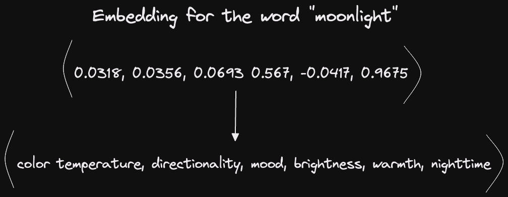
Here we represent a word as an embedding, but equally, an embedding could represent a phrase, sentence, or even a paragraph of text. Typically concepts for a specific dimension are difficult to reason about or attach a label, especially in higher dimensions, but allow words to be conceptually understood when combined. Possibly more importantly, vectors can also be used to represent other data types, such as images and audio. This opens up the possibility of searching formats that were historically challenging for an inverted index-based approach.
Why are vectors and embeddings useful?
Encoding images or text to these common representations allow comparisons between them and the information they represent, even though the original forms of the content were different.
To understand how vector embeddings can be compared to one another, we can picture an embedding as a single point in high-dimensional space. Two embeddings would be two points in this space. If those two embeddings represent conceptually similar objects to one another, these points in space will be geometrically close in distance and angle.
For two or three dimensions, we can easily visualize and comprehend this distance. Below, we assume the concepts for three words “moonlight”, “flashlight and “animal” could be effectively represented in 3 dimensions:
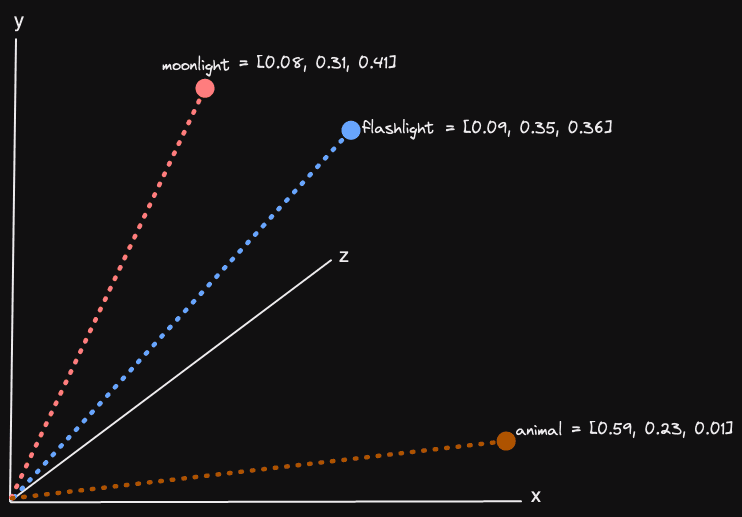
Unfortunately, three dimensions are insufficient to encode all of the concepts in a sizable amount of text, let alone images! Fortunately, the math (Cosine similarity or Euclidean distance usually) that is used to compute the angle or distance between two vectors scales to N dimensions even if we as humans can’t visually comprehend it. Embeddings typically have a dimensionality of under 1000 - more than sufficient to encode most of the concepts in a text corpus. This, of course, assumes we can choose our concepts well and encode our embedding into the space accurately.
It’s estimated that up to 80% to 90% of all data is unstructured. And so, this comparison capability has provided the foundation for algorithms such as neural networks and LLMs to process a class that was historically challenging and costly for businesses to extract insight and from which to base decisions.
Performing vector search
For now, assume we have a means of producing these embeddings using an algorithm, and have done so for all the text we’d like to make searchable. Doing so leaves us with a set of embeddings, potentially in the hundreds of millions, if not billions, in length.
When a user wants to search this repository of text (for which we now have the corresponding embeddings), the user’s search needs to be converted into an embedding itself. Then, the user’s search embedding can be compared with the text repository’s set of embeddings to find the closest match. The closest matching embedding, of course, represents the text that most closely aligns with the user’s search.
In its simplest form, a user might simply be searching for the most relevant document or set of documents by ordering by distance, thus replicating a traditional search engine. However, this ability to find conceptually similar contextual documents to a query has value to other machine learning pipelines, including ChatGPT. Remember, embeddings are compared by angle or distance between them, in vector space.
Performing this vector comparative process typically requires a data store that can persist these vectors and then expose a query syntax in which either a vector or potentially raw query input (usually text) can be passed. This has led to the development of vector databases such as Pinecone and Weviate, which beyond simply storing vectors, offer a means of integrating vector generation processes into their data loading pipelines and query syntax - thus automatically performing the embedding encoding process at both data load and query time. In parallel, existing search engines such as Solr and Elasticsearch have added support for Vector search incorporating new functions to allow users to load and search embeddings.
Additionally, traditional databases with full SQL support, such as Postgres and ClickHouse, have added native support for the storage and retrieval of vectors. In Postgres’ case, this is achieved with the pg_vector. ClickHouse supports the store of vectors as an array column type (Array<Float32>), providing functions to compute the distance between a search vector and column values.
Exacting results vs estimation
When utilizing a data store that supports the search of vectors, users are presented with two high-level approaches:
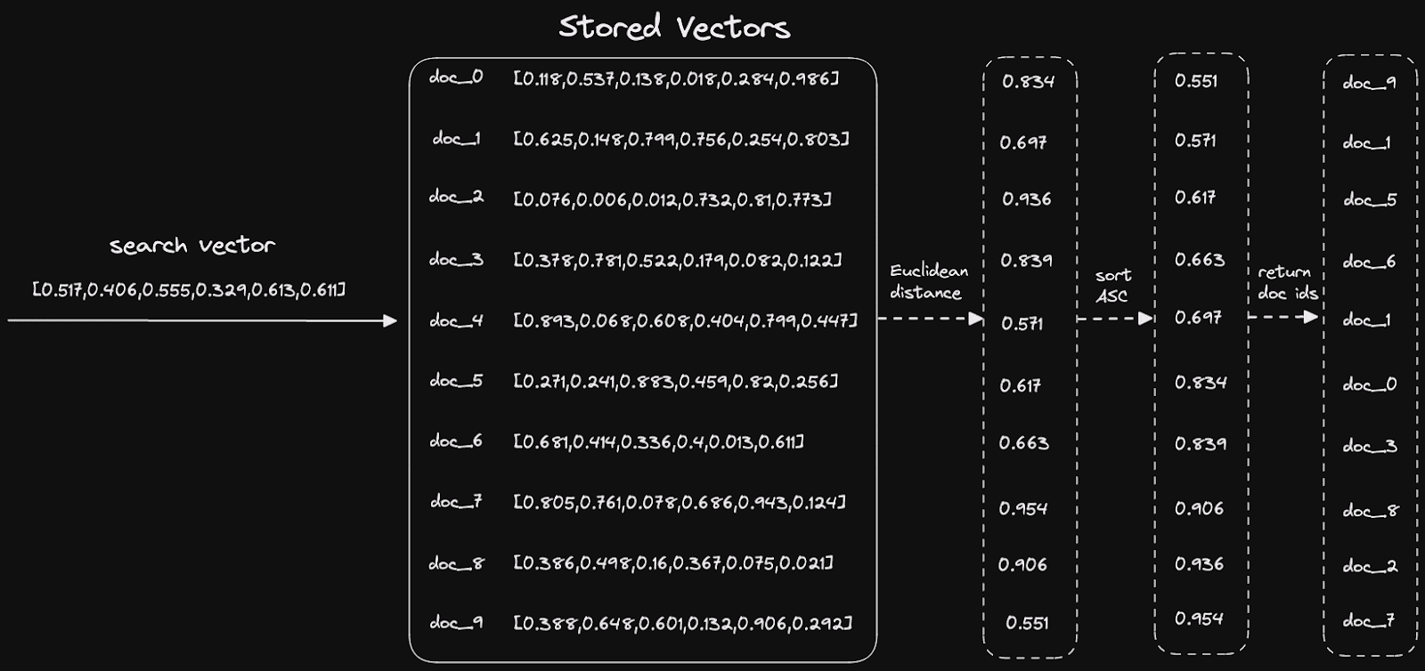
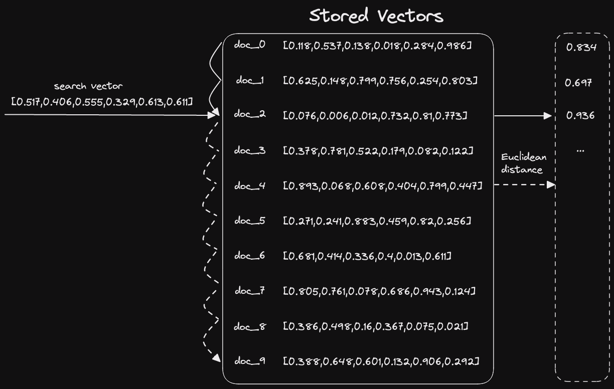
- Exact results with Linear Search - A full comparison of the input vector to every vector in the database, ordering the results by the closest distance and limiting to K hits. This approach, often called K nearest neighbor (KNN), while delivering an exact result with a guarantee of the best quality matches, typically doesn’t easily scale beyond around 100 million without significant parallelization of the matching and/or using GPUs. By its definition, the matching time is directly proportional to the number of vectors that need to be matched (assuming all other variables are constant), i.e., O(n).
- Approximate results with Approximate Nearest Neighbour - While the exact closest matches are sometimes needed, an approximation is often sufficient, especially on larger datasets with many good-quality matches. Algorithms that approximate the best matches are designed to speed up the search process by trading off some level of accuracy by reducing recall for speed. ANN algorithms use various techniques to quickly identify a small subset of the nearest neighbors likely to be the best matches for the query vector. This can significantly reduce the time required to search a large dataset. While ANN algorithms may not always return the exact K nearest neighbors, they are often accurate enough for many applications. ANN algorithms are beneficial in applications where the dataset is large, and the search needs to be performed quickly. Examples here include Hierarchical Navigable Small World (HNSW) and Annoy algorithms.

Annoy algorithm Credit: Alexey Milovidov
The above shows the Annoy algorithm. This works by building a tree-based index on the corpus. This tree structure is built by recursively partitioning the data into smaller subspaces based on the distance metric used (usually Euclidean distance). The partitioning process continues until either the subspaces contain a small number of data points or a certain depth of the tree is reached. When a query is issued the tree is traversed starting from the root node. At each level of the tree, the node closest to the query point is chosen and its child nodes are evaluated. The search continues until a leaf node is reached, which contains a subset of the data points closest to the query point. The nearest neighbors can then be found by computing the distances between the query point and the data points in the leaf node.
Generating embeddings
The detailed process of encoding text, or more rich media such as images, is a large topic that we will defer to a later blog post. In summary, this relies on utilizing machine learning algorithms that recognize content and meaning, producing a mathematical representation for the language or specific domain known as a model. These models can then be used to convert subsequent text (or other assets) to vectors. Transformer-based models are constructs that have proved particularly effective at producing vectors for text-based content. Early versions of this class include the popular BERT model, developed by Google. Transformers themselves are more flexible than simply converting text to vectors and form the foundation for state-of-the-art language translation and the recently popularized chat bot ChatGPT.
As noted earlier, vectors go beyond conceptual embeddings. Users may also choose to construct or add other features to vectors. These can be learned by other models or be carefully selected by experts in a domain who are trying to ensure that the close distance of two vectors captures the meaning of a business problem. See the Applications below for a few examples.
The generation of embeddings for images is also an area of research that has garnered significant attention in recent years, with convolutional neural network architectures dominating with respect to quality when producing embeddings. More recently, Vision Transformers (ViT) have shown promising results for image classification and feature extraction tasks, especially for large-scale datasets.
Multimodal models can work with and encode multiple data types, such as images, text, and audio. These can, for example, generate a vector for both an image and text, effectively producing a joint embedding space where they can both be compared. This can be used to allow users to search using words and find conceptually matching images! OpenAI introduced such an algorithm in 2021 known as CLIP (Contrastive Language-Image Pre-Training). This particular algorithm, whose embeddings we will use in a future post, learns joint representations of images and their associated text captions (provided during training) such that the embeddings of related images and captions are close together in the space. Beyond a simple search case, this allows for tasks such as image captioning and zero-shot image classification.
 Credit: CLIP - https://openai.com/research/clip
Training a model to generate embeddings is, thankfully, not always necessary, as there are now open sourced pre-trained models that can be used to produce such embeddings,downloadable from resources such as Hugging Face These can be adapted to a new domain with minimal additional training in a process known as “transfer learning” or “fine tuning.” Users can also download generated embeddings for a dataset for experimentation. Once a user has generated or downloaded a set of embeddings, a storage medium is typically then required - leading to the adoption of vector databases.
Example applications of vector search
This blog post has focused on introducing the concept of providing semantic search through the generation of vector embeddings, their storage, and retrieval. This capability has a number of applications beyond simply enhancing existing traditional enterprise or application search experiences. Possible uses include, but are not limited to:
- Recommendations - Particularly relevant to e-commerce websites, vector search can be used to find relevant products. Beyond simply embedding text meaning into vectors, features such as page views and past purchases can be encoded in vectors.
- Question answering - Question-answering systems have historically been challenging as users rarely use the same terms as the question. Equivalent meanings can, however, be encoded with vectors that are close, e.g., X and Y.
- Image and video search - Using multimodal models described above, users can search for images and videos based on text - useful for applications such as music and movie recommendation systems, product recommendations, and news article recommendations.
- Fraud detection - We can find similar or dissimilar transactions by encoding users' behaviors or log-in patterns into vectors. These can be anomalous behaviors and prevent fraud.
- Genome analysis - Vector databases can be used to store and retrieve embeddings of genomic sequences, which can be useful for applications such as gene expression analysis, personalized medicine, and drug discovery.
- Multilingual search - Rather than build an index for language (normally an expensive exercise and linear in cost to the number of languages), multilingual models can allow cross-language searching with the same concept in two languages encoded to the same vector.
- Providing context - Recently, vector databases have been leveraged to provide contextual content to chat applications powered by APIs like ChatGPT. For instance, content can be converted to vectors and stored in a vector database. When an end-user asks a question, the database is queried, and relevant documents are identified. Rather than returning these to the user directly, they can be used to provide additional context for ChatGPT to generate a much more robust answer. Our friends at Supabase recently implemented such an architecture to provide a chatbot for their documentation.
Conclusion
In this post, we’ve provided a high-level introduction to vector embeddings and vector databases. We’ve covered their value and how they relate to more traditional search approaches, as well as general approaches to matching vectors at scale - either exactly, or through approximation.
In our next post, we’ll explore practical examples with ClickHouse and answer the question, “When do I use ClickHouse for vector search?”.
For further reading on the history of computational language understanding, we recommend this post.
Get started with ClickHouse Cloud today and receive $300 in credits. At the end of your 30-day trial, continue with a pay-as-you-go plan, or contact us to learn more about our volume-based discounts. Visit our pricing page for details.