Join me if you can: ClickHouse vs. Databricks & Snowflake - Part 2

TL;DR

Replacing joins with in-memory dictionaries in ClickHouse Cloud gave us up to 6.6× faster query times and 60% lower cost, requiring only minor edits to the SQL.

This post walks through the tuning technique (dictionaries), how to use them for dimension table lookups, and real benchmark results from queries over 1.4 billion rows.

Charts for other dataset sizes are in GitHub.

If you’re joining us here first, no worries. Joins in ClickHouse already perform great with zero tuning. In Part 1, we ran 17 join-heavy queries with no tweaks, and ClickHouse still came out ahead: faster and cheaper than Databricks and Snowflake.

This post is about going one step further. If you want even more speed, ClickHouse-native dictionaries can get you there, fast, cheap, and with minimal effort.

So now you might be wondering… should I migrate?

The good news: it’s low friction. In Part 1, we simply created tables with a matching schema and loaded the data directly from external Iceberg tables. (It could’ve been Delta Lake or just Parquet on S3.) The join queries ran unmodified, fast and cheap, right out of the gate.

But why stop there? Let’s see how far we can push performance with a little ClickHouse-native tuning.

In this post, we’ll show how turning your dimension tables into in-memory dictionaries can supercharge your queries. It’s one of the easiest ways to turbocharge join lookups, and it’s a drop-in change that can unlock serious performance gains.

Let’s dive in.

Let’s introduce the star of this tuning technique: dictionaries.

If you’re running queries with joins, especially foreign key joins on small dimension tables in star or snowflake schemas, dictionaries can make a big difference.

Dictionaries let you load a table into memory as a fast, key-value structure, optimized for ultra-low-latency lookups. When one side of a join fits into memory (like a dimension table), you can replace a traditional join with a dictionary lookup and get a speed boost in return.

Let’s revisit the benchmark setup.

The original dataset simulates orders at a national coffee chain and consists of:

• Sales: the main fact table (orders)
• Products: a product dimension table
• Locations: a store/location dimension table

These were the same tables we used in Part 1, and most of the queries rely on foreign key joins, typically between the large fact table and smaller dimension tables, making them ideal for in-memory dictionaries.

Instead of joining against tables on disk, we’ll load the Products and Locations tables into dictionaries, and show how this simple tuning step unlocks even faster performance.

Let’s walk through how to turn your existing dimension tables into dictionaries.

ClickHouse dictionaries are incredibly flexible; you can build them from virtually any source ClickHouse can query. You can load them from any format or location that ClickHouse can read from, which includes a wide range of file formats (like Parquet, Arrow, JSON) and integration points (like S3, HDFS, Kafka, and tables in open formats like Iceberg or Delta Lake). If ClickHouse can query it, you can likely build a dictionary from it.

We’re migrating the Locations dimension table from an existing Iceberg table in S3:

CREATE DICTIONARY dicts.dict_locations
(
    location_id String,
    record_id   String,
    city        String,
    state       String,
    country     String,
    region      String
)
PRIMARY KEY location_id
SOURCE(CLICKHOUSE(
         QUERY "
            SELECT
                COALESCE(location_id, '') AS location_id,
                COALESCE(record_id, '') AS record_id,
                COALESCE(city, '') AS city,
                COALESCE(state, '') AS state,
                COALESCE(country, '') AS country,
                COALESCE(region, '') AS region
            FROM icebergS3('s3://clickhouse-datasets/coffeeshop/dim_locations/')"))
LIFETIME(0)
LAYOUT(complex_key_hashed());

This dict_locations dictionary loads from an external Iceberg table and will be automatically available on all ClickHouse Cloud compute nodes. We set the LIFETIME to 0 to indicate that the content is static and won’t be automatically refreshed.

All lookups into the Locations dimension table in the benchmark queries are simple key lookups by location_id (e.g. 'AUSTX156' or 'HOUTX133'). We use the complex_key_hashed dictionary layout to support fast in-memory access with String keys, since layouts like flat and hashed only support UInt64 keys.

The dictionary layout defines how content is stored in memory, optimized for specific lookup patterns.

To give a second source data example, we’re migrating the Products dimension table directly from its native MergeTree table used in Part 1:

CREATE OR REPLACE DICTIONARY dicts.dict_products (
    record_id String,
    product_id String,
    name String,
    category String,
    subcategory String,
    standard_cost Float64,
    standard_price Float64,
    from_date Date,
    to_date Date
)
PRIMARY KEY name
SOURCE(CLICKHOUSE(db 'coffeeshop' table 'dim_products'))
LIFETIME(0)
LAYOUT(COMPLEX_KEY_RANGE_HASHED())
RANGE(MIN from_date MAX to_date);

All lookups into the Products dimension table in the benchmark queries are range-based using from_date and to_date to find which product version was active at a given time (e.g. as seen in Q4).

To handle this efficiently, we use a Range Dictionary. It’s optimized for exactly this use case: matching a given key and a time to the correct product version. In memory, ClickHouse builds a hash map on the primary key and performs a fast binary search across sorted date ranges.

Just one catch: make sure the source data has no overlapping ranges for the same key, otherwise, the dictionary will only return the first match, which may not be correct. We checked that there are no overlapping ranges in the original Products dimension table.

ClickHouse supports more dictionary layouts for advanced use cases. Like regex matching, CIDR range lookup, or point-in-polygon geospatial queries. We won’t use them here, but if you’re classifying user agents, geolocating IPs, or mapping GPS points, they’re worth checking out.

Once the dictionaries are set up, updating the queries is straightforward. Each join becomes a lightning-fast in-memory lookup. Here’s how we transformed the joins:

SELECT
     f.order_date,
     l.city,
     p.subcategory
   FROM fact_sales f
① JOIN dim_locations l
     ON f.location_id = l.location_id
② JOIN dim_products p
     ON f.product_name = p.name
    AND f.order_date BETWEEN p.from_date AND p.to_date
   WHERE …
   GROUP BY …
   ORDER BY …

The Sales fact table is joined with:

① The Locations dimension table using location_id as join key

② The Products dimension table using a join key combination of product_name and a date range filter (order_date BETWEEN from_date AND to_date)

We swap the two JOINs from above with two dictionary lookups:

SELECT
     f.order_date,
①   dictGet(
       'dicts.dict_locations', 'city',
       f.location_id) AS city,
②   dictGet(
       'dicts.dict_products','subcategory',
       f.product_name, f.order_date) AS subcategory,
   FROM fact_sales f
   WHERE …
   GROUP BY …
   ORDER BY …

① A straightforward one-to-one lookup in the dict_locations dictionary using location_id as the key.
→ This replaces a simple equality join with an in-memory dictionary lookup.

② A range-based lookup in the dict_products dictionary using a compound key of product_name and order_date.
→ This replaces a join with a range predicate (order_date BETWEEN from_date AND to_date) and ensures the correct product version is returned based on time.

These small changes remove full joins from the query plan, replacing them with ultra-fast lookups in memory. The pattern is repeatable and easy to apply across all 17 benchmark queries.

With all the dimension lookups swapped to dictionaries, and the queries adapted, we re-ran the benchmark queries. Let’s see how much performance we gained.

As a reminder, we ran the benchmark using ClickHouse Cloud services, varying the number of compute nodes (which also let us test ClickHouse Cloud’s Parallel Replicas feature). All service configurations used 30 cores and 120 GB RAM per node. The chart labels below follow this format:

CH 2n_30c_120g, where:

• 2n = number of compute nodes

• 30c = CPU cores per node

• 120g = RAM per node (in GB)

To keep things focused, we’re only showing results for the 1b scale (1.4 billion rows in the fact table). Charts for the 500m and 5b scales are available in the GitHub repository.

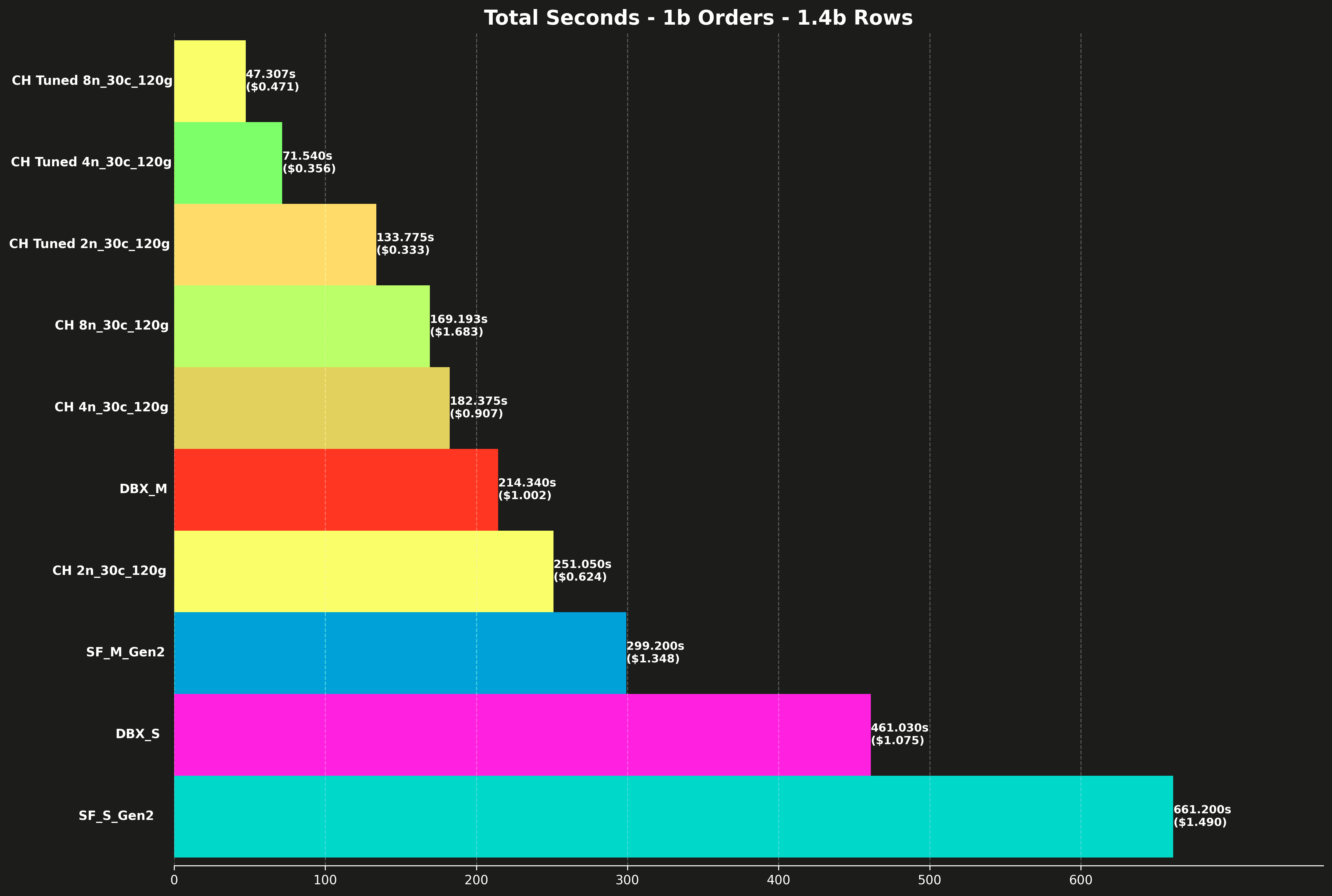
As in Part 1, the chart below shows the total runtime (in seconds) per system for running all 17 benchmark queries sequentially. Each bar also includes the total cost to run all queries, shown in parentheses.

Here’s how tuned ClickHouse stacks up against its untuned baseline, same compute, same dataset, just faster queries:

• 2 nodes (2n_30c_120g)

  • Untuned: 251.05s
  • Tuned: 133.78s
    → That’s a 1.9× speedup, and cuts costs by 47% just by switching from joins to dictionaries.

• 4 nodes (4n_30c_120g)

  • Untuned: 182.38s
  • Tuned: 71.54s
    → A 2.5× speedup, and it also cuts costs by over 60% ($0.907 → $0.356).

• 8 nodes (8n_30c_120g)

  • Untuned: 169.19s
  • Tuned: 47.31s
    → A 3.5× speedup, and the cost is cut by 44%. It’s also cheaper than the fastest non-ClickHouse service, while being dramatically faster.

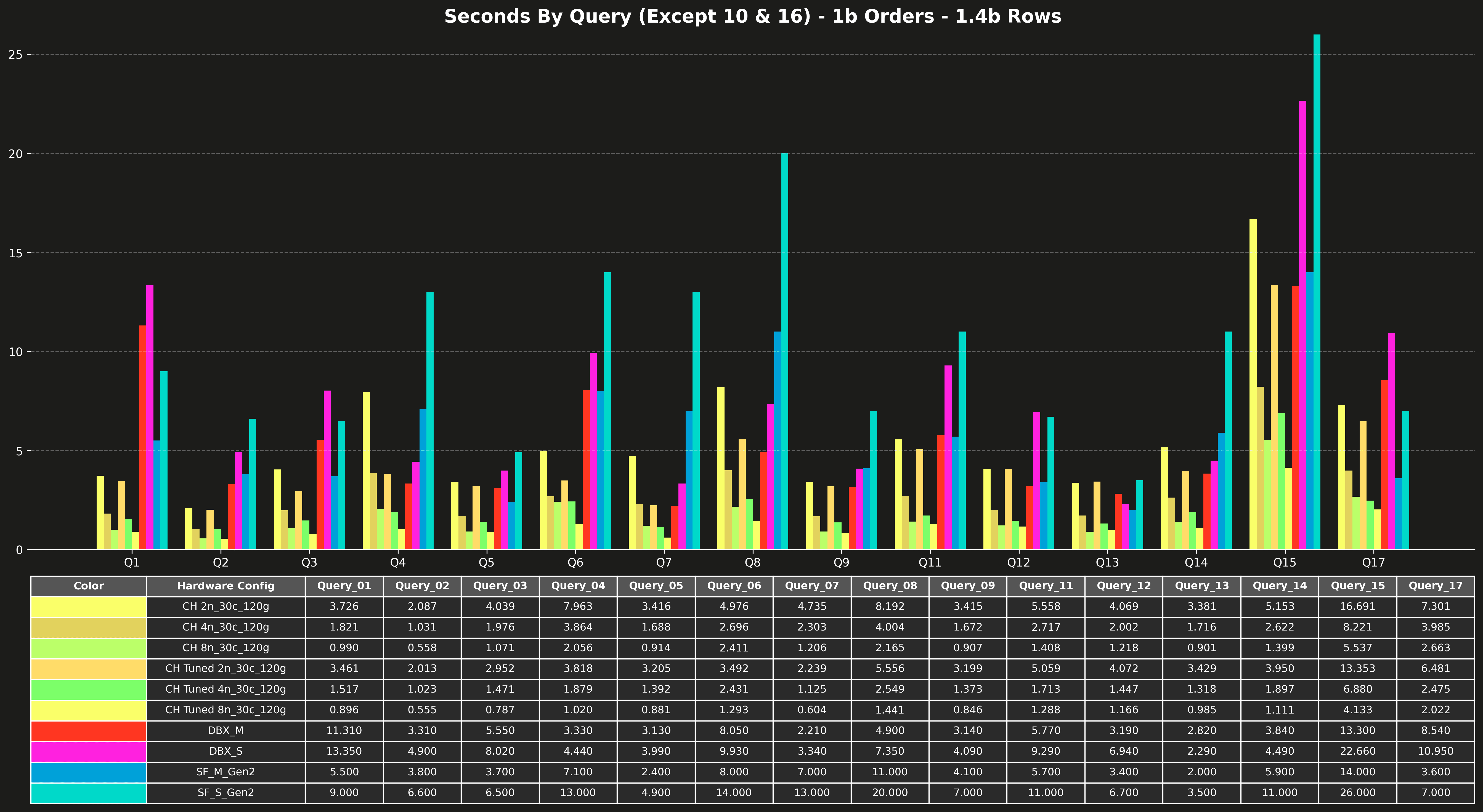
The next chart breaks down the total runtime into individual query runtimes.

Let’s break down a few standout queries where dictionaries had the biggest impact:

Q04

• 2n: 7.96s → 2.95s
• 4n: 3.86s → 1.47s
• 8n: 2.06s → 0.79s
  → ~2.5–3× speedup, a huge benefit from replacing the join with a dictionary

Q08

• 2n: 8.19s → 3.55s
• 4n: 4.00s → 2.55s
• 8n: 2.17s → 1.29s
  → Big gains: ~2–2.7× faster

Q15

• 2n: 16.69s → 6.48s
• 4n: 8.22s → 3.95s
• 8n: 5.54s → 2.02s
  → ~2–3× speedup, particularly impressive at 2 and 8 nodes

Q17

• 2n: 7.30s → 3.95s
• 4n: 3.99s → 2.48s
• 8n: 2.66s → 1.37s
  → Another consistent ~2× gain

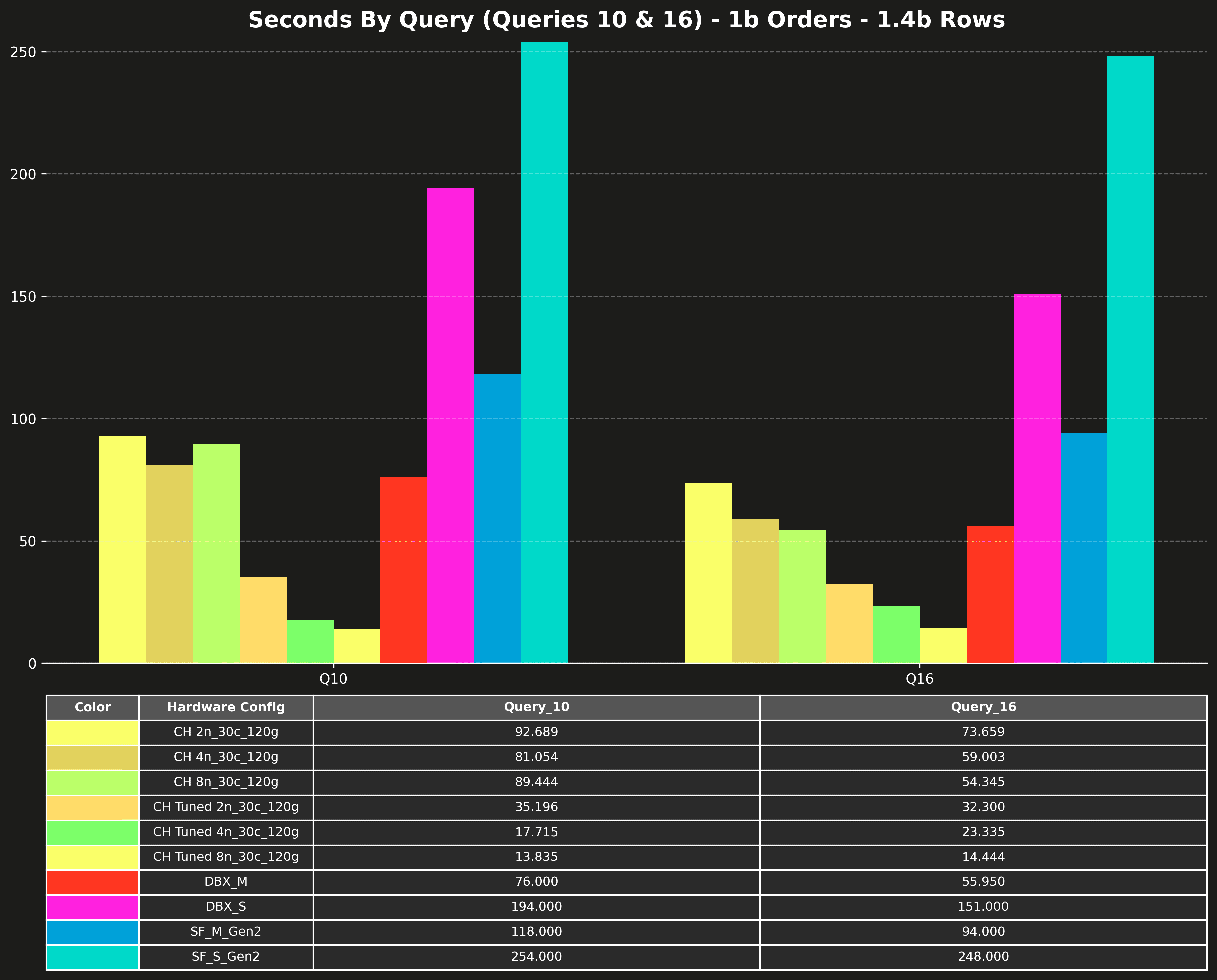
Finally, here’s a separate chart for Q10 and Q16. As noted in Part 1, these two are outliers, much slower than the others, and would distort the scale of the full chart. That’s why the original posts broke them out separately.

Here’s how much tuning improved performance for Query 10 and 16:

Query 10: Large join + filtering

• 2n config: From 92.69s → 35.20s
  → ~2.6× speedup

• 4n config: From 81.05s → 17.72s
  → ~4.6× speedup

• 8n config: From 89.44s → 13.84s,
  → ~6.6× speedup, faster than anything else on the chart

Query 16: Complex, expensive join

• 2n config: From 73.66s → 32.30s
  → ~2.3× speedup

• 4n config: From 59.00s → 23.34s
  → ~2.5× speedup

• 8n config: From 54.35s → 14.44s
  → ~3.7× speedup, once again the fastest overall

ClickHouse was already fast out of the box. But with a few targeted changes, replacing traditional joins with in-memory dictionaries, we made it both faster and cheaper.

• On join-heavy queries, we saw speedups of up to 6.6× and cost savings of over 60%.

• Even the largest, most complex queries (like Q10 and Q16) finished minutes faster with simple dictionary lookups.

• These improvements required no data reloading, no schema rewrites, and scaled cleanly from 2 nodes to 8.

If you’re running joins against dimension tables, dictionaries are a no-brainer. They’re fast, flexible, and require almost no friction to adopt. And if you’re evaluating ClickHouse, this is your sign: the engine isn’t just fast, it keeps getting faster the more you use it.