Another month goes by, which means it’s time for another release!
ClickHouse version 24.6 contains 23 new features 🎁 24 performance optimisations 🛷 59 bug fixes 🐛
New Contributors
As always, we send a special welcome to all the new contributors in 24.6! ClickHouse's popularity is, in large part, due to the efforts of the community that contributes. Seeing that community grow is always humbling.
Below are the names of the new contributors:
Artem Mustafin, Danila Puzov, Francesco Ciocchetti, Grigorii Sokolik, HappenLee, Kris Buytaert, Lee sungju, Mikhail Gorshkov, Philipp Schreiber, Pratima Patel, Sariel, TTPO100AJIEX, Tim MacDonald, Xu Jia, ZhiHong Zhang, allegrinisante, anonymous, chloro, haohang, iceFireser, morning-color, pn, sarielwxm, wudidapaopao, xogoodnow
Hint: if you’re curious how we generate this list… click here.
You can also view the slides from the presentation.
Optimal Table Sorting
Contributed by Igor Markelov
The physical on-disk order of rows in MergeTree tables is defined by their ORDER BY key.
As a reminder, the ORDER BY key and the related physical row order have three purposes:
- To build a sparse index for range requests (can also be specified as PRIMARY KEY).
- To define a key for merging modes, e.g. for Aggregating- or ReplacingMergeTree tables.
- To provide a way to improve compression by co-locating data in column files.
For the third purpose mentioned above, this release introduces a new setting called optimize_row_order. This setting is available exclusively for ordinary MergeTree-engine tables. After sorting by the ORDER BY column(s), it automatically sorts the table rows during ingestion by the remaining columns based on their cardinality, ensuring optimal compression.
Generic compression codecs such as LZ4 and ZSTD achieve maximum compression rates if the data exposes patterns. For example, long runs of the same value typically compress very well. Such long runs of the same value can be achieved by physically storing the rows sorted by column values, starting with the lowest cardinality columns. The following diagram illustrates this:

Because the rows in the diagram above are sorted on disk by column values starting with the lowest cardinality columns, there are long runs of the same values per column. As mentioned above, this benefits the compression ratio of the table part’s column files.
As a counter-example, the next figure illustrates the effect of sorting rows on disk by a high cardinality column first:

Because the rows are ordered by high cardinality column values first, it is generally no longer possible to sort the rows based on the other column’s values to create long runs of the same values. Therefore the compression ratio of the column files is suboptimal.
With the new optimize_row_order setting, ClickHouse automatically achieves optimal data compression. ClickHouse stores the rows on disk first sorted (as usual) by the ORDER BY columns. Additionally, per range of rows with the same ORDER BY column values, the rows are sorted by the values of the remaining columns ordered by range-local column-cardinality in ascending order:

This optimization is only applied for data parts created at insert time but not during part merges. As most merges of ordinary MergeTree tables simply concatenate non-overlapping ranges of the ORDER BY key, the already optimized row order is generally retained.
INSERTs are expected to take 30-50% longer, depending on the data characteristics.
Compression rates of LZ4 or ZSTD are expected to improve by 20-40% on average.
This setting works best for tables with no ORDER BY key or a low-cardinality ORDER BY key, i.e. a table with only a few distinct ORDER BY key values. Tables with high-cardinality ORDER BY keys, e.g., timestamp columns of type DateTime64, are not expected to benefit from this setting.
To demonstrate this new optimization, we load 1 billion rows of the public PyPI download statistics data set into a table without and a table with the optimize_row_order setting.
We create the table without the new setting:
CREATE OR REPLACE TABLE pypi
(
`timestamp` DateTime64(6),
`date` Date MATERIALIZED timestamp,
`country_code` LowCardinality(String),
`url` String,
`project` String,
`file` Tuple(filename String, project String, version String, type Enum8('bdist_wheel' = 0, 'sdist' = 1, 'bdist_egg' = 2, 'bdist_wininst' = 3, 'bdist_dumb' = 4, 'bdist_msi' = 5, 'bdist_rpm' = 6, 'bdist_dmg' = 7)),
`installer` Tuple(name LowCardinality(String), version LowCardinality(String)),
`python` LowCardinality(String),
`implementation` Tuple(name LowCardinality(String), version LowCardinality(String)),
`distro` Tuple(name LowCardinality(String), version LowCardinality(String), id LowCardinality(String), libc Tuple(lib Enum8('' = 0, 'glibc' = 1, 'libc' = 2), version LowCardinality(String))),
`system` Tuple(name LowCardinality(String), release String),
`cpu` LowCardinality(String),
`openssl_version` LowCardinality(String),
`setuptools_version` LowCardinality(String),
`rustc_version` LowCardinality(String),
`tls_protocol` Enum8('TLSv1.2' = 0, 'TLSv1.3' = 1),
`tls_cipher` Enum8('ECDHE-RSA-AES128-GCM-SHA256' = 0, 'ECDHE-RSA-CHACHA20-POLY1305' = 1, 'ECDHE-RSA-AES128-SHA256' = 2, 'TLS_AES_256_GCM_SHA384' = 3, 'AES128-GCM-SHA256' = 4, 'TLS_AES_128_GCM_SHA256' = 5, 'ECDHE-RSA-AES256-GCM-SHA384' = 6, 'AES128-SHA' = 7, 'ECDHE-RSA-AES128-SHA' = 8, 'AES128-GCM' = 9)
)
Engine = MergeTree
ORDER BY (project);And load the data into that table. Note that we increased the value of the min_insert_block_size_rows setting to demonstrate the optimization better :
INSERT INTO pypi
SELECT
*
FROM s3(
'https://storage.googleapis.com/clickhouse_public_datasets/pypi/file_downloads/sample/2023/{0..61}-*.parquet')
SETTINGS
input_format_null_as_default = 1,
input_format_parquet_import_nested = 1,
min_insert_block_size_bytes = 0,
min_insert_block_size_rows = 60_000_000;Next we create the same table with the new setting:
CREATE TABLE pypi_opt
(
`timestamp` DateTime64(6),
`date` Date MATERIALIZED timestamp,
`country_code` LowCardinality(String),
`url` String,
`project` String,
`file` Tuple(filename String, project String, version String, type Enum8('bdist_wheel' = 0, 'sdist' = 1, 'bdist_egg' = 2, 'bdist_wininst' = 3, 'bdist_dumb' = 4, 'bdist_msi' = 5, 'bdist_rpm' = 6, 'bdist_dmg' = 7)),
`installer` Tuple(name LowCardinality(String), version LowCardinality(String)),
`python` LowCardinality(String),
`implementation` Tuple(name LowCardinality(String), version LowCardinality(String)),
`distro` Tuple(name LowCardinality(String), version LowCardinality(String), id LowCardinality(String), libc Tuple(lib Enum8('' = 0, 'glibc' = 1, 'libc' = 2), version LowCardinality(String))),
`system` Tuple(name LowCardinality(String), release String),
`cpu` LowCardinality(String),
`openssl_version` LowCardinality(String),
`setuptools_version` LowCardinality(String),
`rustc_version` LowCardinality(String),
`tls_protocol` Enum8('TLSv1.2' = 0, 'TLSv1.3' = 1),
`tls_cipher` Enum8('ECDHE-RSA-AES128-GCM-SHA256' = 0, 'ECDHE-RSA-CHACHA20-POLY1305' = 1, 'ECDHE-RSA-AES128-SHA256' = 2, 'TLS_AES_256_GCM_SHA384' = 3, 'AES128-GCM-SHA256' = 4, 'TLS_AES_128_GCM_SHA256' = 5, 'ECDHE-RSA-AES256-GCM-SHA384' = 6, 'AES128-SHA' = 7, 'ECDHE-RSA-AES128-SHA' = 8, 'AES128-GCM' = 9)
)
Engine = MergeTree
ORDER BY (project)
SETTINGS optimize_row_order = 1;And load the data into the table:
INSERT INTO pypi_opt
SELECT
*
FROM s3(
'https://storage.googleapis.com/clickhouse_public_datasets/pypi/file_downloads/sample/2023/{0..61}-*.parquet')
SETTINGS
input_format_null_as_default = 1,
input_format_parquet_import_nested = 1,
min_insert_block_size_bytes = 0,
min_insert_block_size_rows = 60_000_000;Let’s compare the storage size and compression ratios of both tables:
SELECT
`table`,
formatReadableQuantity(sum(rows)) AS rows,
formatReadableSize(sum(data_uncompressed_bytes)) AS uncompressed,
formatReadableSize(sum(data_compressed_bytes)) AS compressed,
round(sum(data_uncompressed_bytes) / sum(data_compressed_bytes), 0) AS ratio
FROM system.parts
WHERE active AND (database = 'default') AND startsWith(`table`, 'pypi')
GROUP BY `table`
ORDER BY `table` ASC;
┌─table────┬─rows─────────┬─uncompressed─┬─compressed─┬─ratio─┐
1. │ pypi │ 1.01 billion │ 227.97 GiB │ 25.36 GiB │ 9 │
2. │ pypi_opt │ 1.01 billion │ 227.97 GiB │ 17.52 GiB │ 13 │
└──────────┴──────────────┴──────────────┴────────────┴───────┘As you can see, the data compression improved by ~30% for the table with the new setting.
chDB 2.0
Contributed by Auxten Wang
chDB is a n in-process version of ClickHouse for various languages, most prominently Python. It joined the ClickHouse family earlier this year and released a beta 2.0 release of the Python library this week.
To install that version, you’ll have to specify the version during installation like this:
pip install chdb==2.0.0b1In this version, the ClickHouse engine is upgraded to version 24.5, and it’s now possible to query Pandas DataFrames, Arrow tables, and Python objects directly.
Let’s start by generating a CSV file that contains 100 million rows:
import pandas as pd
import datetime as dt
import random
rows = 100_000_000
now = dt.date.today()
df = pd.DataFrame({
"score": [random.randint(0, 1_000_000) for _ in range(0, rows)],
"result": [random.choice(['win', 'lose', 'draw']) for _ in range(0, rows)],
"dateOfBirth": [now - dt.timedelta(days = random.randint(5_000, 30_000)) for _ in range(0, rows)]
})
df.to_csv("scores.csv", index=False)We can then write the following code to load the data back into a Pandas DataFrame and query the DataFrame using chDB’s Python table engine:
import pandas as pd
import chdb
import time
df = pd.read_csv("scores.csv")
start = time.time()
print(chdb.query("""
SELECT sum(score), avg(score), median(score),
avgIf(score, dateOfBirth > '1980-01-01') as avgIf,
countIf(result = 'win') AS wins,
countIf(result = 'draw') AS draws,
countIf(result = 'lose') AS losses,
count()
FROM Python(df)
""", "Vertical"))
end = time.time()
print(f"{end-start} seconds")The output is as follows:
Row 1:
──────
sum(score): 49998155002154
avg(score): 499981.55002154
median(score): 508259
avgIf: 499938.84709508
wins: 33340305
draws: 33334238
losses: 33325457
count(): 100000000
0.4595322608947754 secondsWe could load the CSV file into a PyArrow table and query that table:
import pyarrow.csv
table = pyarrow.csv.read_csv("scores.csv")
start = time.time()
print(chdb.query("""
SELECT sum(score), avg(score), median(score),
avgIf(score, dateOfBirth > '1980-01-01') as avgIf,
countIf(result = 'win') AS wins,
countIf(result = 'draw') AS draws,
countIf(result = 'lose') AS losses,
count()
FROM Python(table)
""", "Vertical"))
end = time.time()
print(f"{end-start} seconds")The output of that code block is shown below:
Row 1:
──────
sum(score): 49998155002154
avg(score): 499981.55002154
median(score): 493265
avgIf: 499955.15289763256
wins: 33340305
draws: 33334238
losses: 33325457
count(): 100000000
3.0047709941864014 secondsWe can also query Python dictionaries as long as the value is a list:
x = {"col1": [random.uniform(0, 1) for _ in range(0, 1_000_000)]}
print(chdb.query("""
SELECT avg(col1), max(col1)
FROM Python(x)
""", "DataFrame"))
avg(col1) max(col1)
0 0.499888 0.999996Give it a try, and let us know how you get on!
Hilbert Curves
Contributed by Artem Mustafin
Users with a background in mathematics may be familiar with the concept of space-filling curves. In 24.6, we have added support for Hilbert curves to complement the existing Morton encoding functions. These offer the potential to accelerate certain queries, which can be common in time series and geographical data.
Space-filling curves are continuous curves that pass through every point in a given multidimensional space, typically within a unit square or cube, thereby completely filling the space. These curves are fascinating for many, primarily because they defy the intuitive notion that a one-dimensional line cannot cover a two-dimensional area or a higher-dimensional volume. The most famous examples include the Hilbert curve and the simpler (and slightly earlier) Peano curve, both of which are constructed iteratively to increase their complexity and density within the space. Space-filling curves have practical applications in databases, as they provide an effective way to map multidimensional data into one dimension while preserving locality.
Consider a 2-dimensional coordinate system where a function maps any point to a 1-dimensional line while preserving locality, ensuring points close in the original space remain close on the line. This line orders high-dimensional data with a single numerical value. Visualize this by imagining a 2-dimensional space divided into four quadrants, each further split into four, resulting in 16 parts. This recursive process, though conceptually infinite, is easier to grasp at a finite depth, such as depth 3, yielding an 8x8 grid with 64 quadrants. The curve produced by this function passes through all quadrants, maintaining proximity of original points on the final line.

Importantly, the deeper we recurse and spit the space, the more points on the line stabilize in their equivalent 2 dimensional location. At infinity the space is fully “filled”.
Users may also be familiar with the term Z-ordering from lake formats such as Delta lake - also known as the Morton order. This is another type of space-filling curve which also preserves spatial locality, similar to our Hilbert example above. The Morton order, supported through a mortenEncode function in Clickhouse, does not preserve locality as well as the Hilbert curve but is often preferred in certain contexts due to its simpler computation and implementation.
For a fantastic introduction to space filling curves and their relation to infinite math, we recommend this video.
So why might this be useful in optimizing queries in a database?
We can effectively encode multiple columns as a single value and by maintaining the spatial locality of the data, use the resulting value as a sort order in our table. This can be useful in improving the performance of range queries and nearest neighbor searches and is most effective when the encoded columns have similar properties in terms of range and distribution while also having a high number of distinct values. The discussed properties of the space-filling curve ensure values that are close in high dimensional space which the same range query will match, will have a similar sort value, and will be part of the same granules. As a result, fewer granules need to be read, and queries will be faster!
The columns should also not be correlated - traditional lexicographical ordering, as used by ClickHouse ordering keys, is more efficient in this case as sorting by the first column will sort the 2nd inherently.
While numerical IOT data, such as timestamps and sensor values, typically satisfy these properties, the more intuitive example is geographical latitude and longitude coordinates. Let's look at a simple example of how Hilbert encoding can be used to accelerate these types of queries.
Consider the NOAA Global Historical Climatology Network data, containing 1 billion weather measurements for the last 120 years. Each row is a measurement for a point in time and station. We perform the following on a 2xcore r5.large instance.
We have modified the default schema slightly, adding the mercator_x and mercator_y columns. These values result from a Mercator projection of the latitude and longitude values, implemented as a UDF, allowing the data to be visualized on a 2d surface. This projection is typically used to project points into a pixel space of a specified height and width, as demonstrated in previous blogs. We use this to project our coordinates from a Float32 to an unsigned integer (using the maximum Int32 value of 4294967295 as our height and width), as required by our hilbertEncode function.
The Mercator projector is a popular projection often used for maps. This has a number of advantages; principally, it preserves angles and shapes at a local scale, making it an excellent choice for navigation. It also has the advantage that constant bearings (directions of travel) are straight lines, making navigating simple.
CREATE OR REPLACE FUNCTION mercator AS (coord) -> (
((coord.1) + 180) * (4294967295 / 360),
(4294967295 / 2) - ((4294967295 * ln(tan((pi() / 4) + ((((coord.2) * pi()) / 180) / 2)))) / (2 * pi()))
)
CREATE TABLE noaa
(
`station_id` LowCardinality(String),
`date` Date32,
`tempAvg` Int32 COMMENT 'Average temperature (tenths of a degrees C)',
`tempMax` Int32 COMMENT 'Maximum temperature (tenths of degrees C)',
`tempMin` Int32 COMMENT 'Minimum temperature (tenths of degrees C)',
`precipitation` UInt32 COMMENT 'Precipitation (tenths of mm)',
`snowfall` UInt32 COMMENT 'Snowfall (mm)',
`snowDepth` UInt32 COMMENT 'Snow depth (mm)',
`percentDailySun` UInt8 COMMENT 'Daily percent of possible sunshine (percent)',
`averageWindSpeed` UInt32 COMMENT 'Average daily wind speed (tenths of meters per second)',
`maxWindSpeed` UInt32 COMMENT 'Peak gust wind speed (tenths of meters per second)',
`weatherType` Enum8('Normal' = 0, 'Fog' = 1, 'Heavy Fog' = 2, 'Thunder' = 3, 'Small Hail' = 4, 'Hail' = 5, 'Glaze' = 6, 'Dust/Ash' = 7, 'Smoke/Haze' = 8, 'Blowing/Drifting Snow' = 9, 'Tornado' = 10, 'High Winds' = 11, 'Blowing Spray' = 12, 'Mist' = 13, 'Drizzle' = 14, 'Freezing Drizzle' = 15, 'Rain' = 16, 'Freezing Rain' = 17, 'Snow' = 18, 'Unknown Precipitation' = 19, 'Ground Fog' = 21, 'Freezing Fog' = 22),
`location` Point,
`elevation` Float32,
`name` LowCardinality(String),
`mercator_x` UInt32 MATERIALIZED mercator(location).1,
`mercator_y` UInt32 MATERIALIZED mercator(location).2
)
ENGINE = MergeTree
ORDER BY (station_id, date)
INSERT INTO noaa SELECT * FROM s3('https://datasets-documentation.s3.eu-west-3.amazonaws.com/noaa/noaa_enriched.parquet') WHERE location.1 < 180 AND location.1 > -180 AND location.2 > -90 AND location.2 < 90Suppose we wish to compute statistics for an area denoted by a bounding box. As an example, let's calculate the total snowfall and average snow depth for the Alps for each week of the year (maybe giving us an indication of the best time to ski!).

The ordering above (station_id, date) provides no real benefit here and results in a linear scan of all rows.
WITH
mercator((5.152588, 44.184654)) AS bottom_left,
mercator((16.226807, 47.778548)) AS upper_right
SELECT
toWeek(date) AS week,
sum(snowfall) / 10 AS total_snowfall,
avg(snowDepth) AS avg_snowDepth
FROM noaa
WHERE (mercator_x >= (bottom_left.1)) AND (mercator_x < (upper_right.1)) AND (mercator_y >= (upper_right.2)) AND (mercator_y < (bottom_left.2))
GROUP BY week
ORDER BY week ASC
54 rows in set. Elapsed: 1.449 sec. Processed 1.05 billion rows, 4.61 GB (726.45 million rows/s., 3.18 GB/s.)
┌─week─┬─total_snowfall─┬──────avg_snowDepth─┐
│ 0 │ 0 │ 150.52388947519907 │
│ 1 │ 56.7 │ 164.85788967420854 │
│ 2 │ 44 │ 181.53357163761027 │
│ 3 │ 13.3 │ 190.36173190191738 │
│ 4 │ 25.2 │ 199.41843468092216 │
│ 5 │ 30.7 │ 207.35987294422503 │
│ 6 │ 18.8 │ 222.9651218746731 │
│ 7 │ 7.6 │ 233.50080515297907 │
│ 8 │ 2.8 │ 234.66253449285057 │
│ 9 │ 19 │ 231.94969343126792 │
...
│ 48 │ 5.1 │ 89.46301878043126 │
│ 49 │ 31.1 │ 103.70976325737577 │
│ 50 │ 11.2 │ 119.3421940216704 │
│ 51 │ 39 │ 133.65286953585073 │
│ 52 │ 20.6 │ 138.1020341499629 │
│ 53 │ 2 │ 125.68478260869566 │
└─week─┴─total_snowfall──┴──────avg_snowDepth─┘A natural choice for this type of query might be to order the table by (mercator_x, mercator_y) - ordering data first by mercator_x and then mercator_y. This actually delivers a significant improvement in query performance time by reducing the number of rows read to 42 million:
CREATE TABLE noaa_lat_lon
(
`station_id` LowCardinality(String),
…
`mercator_x` UInt32 MATERIALIZED mercator(location).1,
`mercator_y` UInt32 MATERIALIZED mercator(location).2
)
ENGINE = MergeTree
ORDER BY (mercator_x, mercator_y)
--populate from existing
INSERT INTO noaa_lat_lon SELECT * FROM noaa
WITH
mercator((5.152588, 44.184654)) AS bottom_left,
mercator((16.226807, 47.778548)) AS upper_right
SELECT
toWeek(date) AS week,
sum(snowfall) / 10 AS total_snowfall,
avg(snowDepth) AS avg_snowDepth
FROM noaa_lat_lon
WHERE (mercator_x >= (bottom_left.1)) AND (mercator_x < (upper_right.1)) AND (mercator_y >= (upper_right.2)) AND (mercator_y < (bottom_left.2))
GROUP BY week
ORDER BY week ASC
--results omitted for brevity
54 rows in set. Elapsed: 0.197 sec. Processed 42.37 million rows, 213.44 MB (214.70 million rows/s., 1.08 GB/s.)As a side note, experienced ClickHouse users might be tempted to use the function
pointInPolygonhere. This does not unfortunately currently exploit the index and results in slower performance.
We can see this key is relatively effective at filtering granules, reducing the number to read to 5172, by using the EXPLAIN indexes=1 clause.
EXPLAIN indexes = 1
WITH
mercator((5.152588, 44.184654)) AS bottom_left,
mercator((16.226807, 47.778548)) AS upper_right
SELECT
toWeek(date) AS week,
sum(snowfall) / 10 AS total_snowfall,
avg(snowDepth) AS avg_snowDepth
FROM noaa_lat_lon
WHERE (mercator_x >= (bottom_left.1)) AND (mercator_x < (upper_right.1)) AND (mercator_y >= (upper_right.2)) AND (mercator_y < (bottom_left.2))
GROUP BY week
ORDER BY week ASC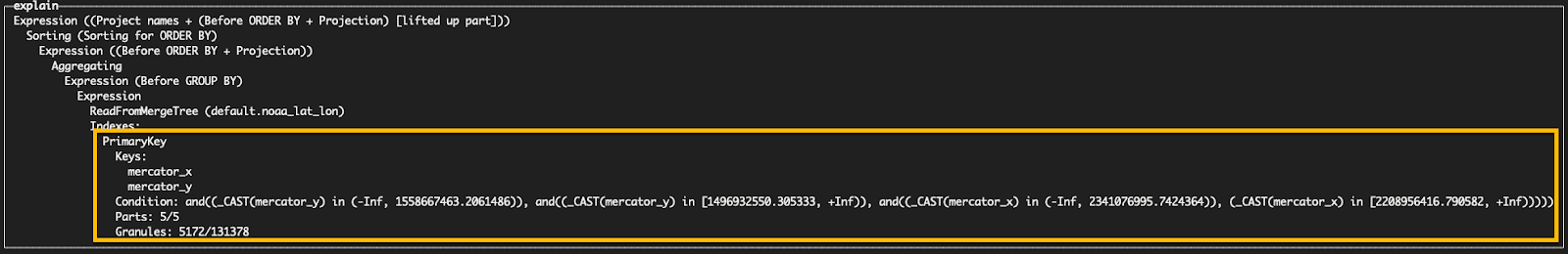
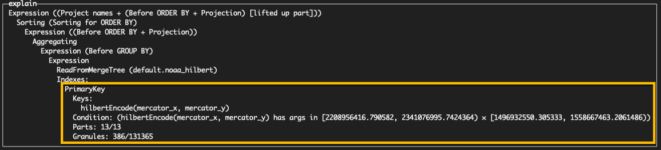
However, the above 2-level sorting does not guarantee points that are in close proximity reside in the same granules. A Hilbert encoding should provide this property, allowing us to filter granules even more effectively. For this, we need to modify the table ORDER BY to hilbertEncode(mercator_x, mercator_y).
CREATE TABLE noaa_hilbert
(
`station_id` LowCardinality(String),
...
`mercator_x` UInt32 MATERIALIZED mercator(location).1,
`mercator_y` UInt32 MATERIALIZED mercator(location).2
)
ENGINE = MergeTree
ORDER BY hilbertEncode(mercator_x, mercator_y)
WITH
mercator((5.152588, 44.184654)) AS bottom_left,
mercator((16.226807, 47.778548)) AS upper_right
SELECT
toWeek(date) AS week,
sum(snowfall) / 10 AS total_snowfall,
avg(snowDepth) AS avg_snowDepth
FROM noaa_hilbert
WHERE (mercator_x >= (bottom_left.1)) AND (mercator_x < (upper_right.1)) AND (mercator_y >= (upper_right.2)) AND (mercator_y < (bottom_left.2))
GROUP BY week
ORDER BY week ASC
--results omitted for brevity
54 rows in set. Elapsed: 0.090 sec. Processed 3.15 million rows, 41.16 MB (35.16 million rows/s., 458.74 MB/s.)Our encoding halves our query performance to 0.09s with only 3m rows read. We can confirm more efficient granule filtering with EXPLAIN indexes=1.
Why not just encode all my ordering keys with Hilbert or Morton encoding?
Firstly, the mortonEncode and hilbertEncode functions are limited to unsigned integers (hence the need to use Mercator projection above). Secondly, as noted, if your columns are correlated, then using a space-filling curve adds no benefit at the additional cost of inserting (and sorting) time overhead. Furthermore, classic ordering is more efficient if just filtering by the first column in the key. A Hilbert (or Morton ordering) encoding will, on average, be faster if filtering by just the 2nd column.